Buprenorphine, an opioid partial agonist, is a medication that works on the same brain receptors as opioids (like heroin or prescription painkillers), but it has a ‘ceiling effect’ that reduces the potential for misuse and overdose.
Buprenorphine is effective in treating opioid use disorder (OUD). It significantly reduces cravings, withdrawal symptoms, and overdose risk, facilitating a more stable lifestyle and aiding recovery efforts.
Buprenorphine is available alone (e.g., Probuphine®, Sublocade™, Bunavail®) or in combination with naloxone (e.g., Suboxone®, Zubsolv®).
Compared to placebo, buprenorphine at appropriate dosages (generally 16mg/day or more) leads to better treatment retention and reduces opioid-positive tests. Extended treatment duration is often crucial. Long-term buprenorphine use (maintenance) often has better outcomes than rapid tapering.
While highly effective, access to buprenorphine has historically been limited (e.g, regulations requiring special training for providers to prescribe, caps on the number of patients providers can treat, regulations requiring special training for providers to prescribe, and stigma surrounding addiction treatment). This is changing due to growing acceptance of medication-assisted treatment (MAT) approaches and federal regulatory changes easing provider restrictions.
Treatment success also often involves behavioral counseling and other recovery support, in addition to medication.
7.2 Public Health Objectives
Reduce barriers to buprenorphine treatment for patients with OUD.
Expand the pool of healthcare providers qualified to prescribe buprenorphine.
Improve accessibility and reach, especially in underserved areas.
7.3 Federal Policies
Here’s a timeline of key policy changes aimed at increasing the availability of buprenorphine treatment:
Drug Addiction Treatment Act of 2000 (DATA 2000)
Established initial framework for office-based buprenorphine treatment, but with strict regulations:
Physician-only prescribing
Mandatory training/waiver
Patient caps limiting provider capacity
Comprehensive Addiction and Recovery Act of 2016 (CARA 2016):
Eased some restrictions under DATA 2000:
Increased patient cap to 100 (after one year)
Allowed prescription by nurse practitioners (NPs) and physician assistants (PAs)
Substance Use Disorder Prevention that Promotes Opioid Recovery and Treatment for Patients and Communities (SUPPORT) Act (SUPPORT 2018):
Further expanded access authorized under CARA 2016:
Practitioners could treat up to 100 patients immediately (with conditions)
Extended prescribing eligibility to other professionals (nurse specialists, midwives, nurse anesthetists)
COVID-19 Pandemic Changes:
DEA allowed buprenorphine prescribing via telemedicine
Waiver training requirements temporarily suspended
7.4 Policy Interventions
In an interrupted time series analysis, we identify specific points where interventions or policy changes occur. For this analysis, we selected the following implementation dates for federal policies, informed by a review of the Federal Register and existing literature:
DATA 2000 Period (55 months): January 2012 to July 2016
CARA (27 months): August 2016 to October 2018
SUPPORT (17 months): November 2018 to February 2020
COVID-19 Period (34 months): March 2020 to December 2022
Additionally, we examined a three-month stay-at-home order period (March to May 2020) as a distinct sub-period within the broader COVID-19 policy changes.
8.0.1 Washington Prescription Monitoring Program (PMP)
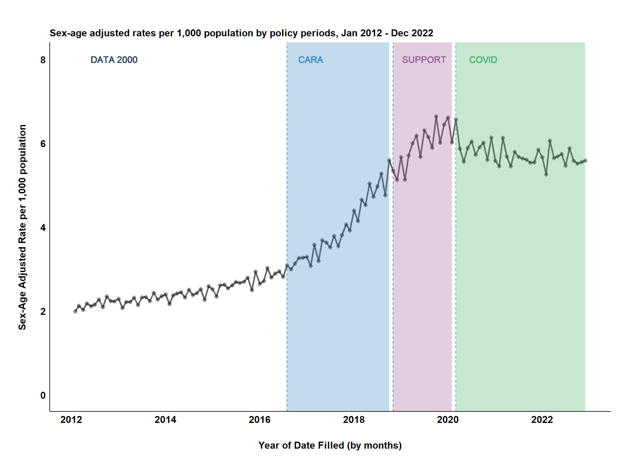
In this example, we are using sex-age adjusted dispensation rates per 1,000 population from the Washington PMP for buprenorphine, a medication used for opioid addiction treatment, from January 2012 to December 2022.
We excluded certain types of buprenorphine prescriptions for pain treatment, prescriptions for animals, those for people living outside Washington State, and any records that were incomplete or had errors.
Notably, buprenorphine prescriptions from certain federal health programs, such as substance use and treatment facilities, are not included in the Washington PMP data. However, this should not affect the purpose of this analysis, which focuses on only buprenorphine dispensations and prescribing that happens outside of these facilities.
8.0.2 Outcome
The sex-age adjusted monthly rate of buprenorphine dispensations per 1,000 people in Washington State, with a specific focus on changes following the implementation of federal policies (CARA, SUPPORT, and subsequent COVID-19 adjustments).
9 Method
9.1 Interrupted Time Series Model
An interrupted time series model is a type of linear regression with multiple terms
Yt: Sex-age adjusted buprenorphine dispensing rate per 1,000 population at time t.
β0: Baseline level of buprenorphine dispensing at the start of the study.
T: Continuous variable for time (e.g., months since the starting period or January 2012).
β1: Baseline trend in dispensing rates before any policy interventions.
CARARamp: Ramp effect variable (0 on and before CARA, increment by 1 for each month after CARA).
β2: Ramp change in dispensing rates associated with CARA’s implementation.
SUPPORTRamp: Ramp effect variable (0 on and before SUPPORT, increment by 1 for each month after SUPPORT).
β3: Ramp change in dispensing rates associated with SUPPORT’s implementation.
COVIDRamp: Ramp effect variable (0 on and before COVID-19 Pandemic Public Health Emergency, increment by 1 for each month after COVID).
β4: Ramp change in dispensing rates associated with COVID’s policy-related changes.
StayAtHome: Step effect dummy variable (0 on and before COVID-19 Pandemic Public Health Emergency, 1 for each month during the three months stay-at-home order during the COVID-19 pandemic).
β5: Step change in dispensing rates associated with COVID’s stay-at-home order.
ϵ: Error term (random variation and other unaccounted factors).
Policy Impact Breakdown
Policies impacting buprenorphine dispensing can have the following effects:
Step Effect (β5): A sustained change in dispensing rates to a new level maintained after the policy is enacted.
Ramp Effect (β2, β3, β4): A gradual increase or decrease in dispensing rates over an extended period following the policy change.
9.1.1 Statistical Hypothesis
Hypotheses about Trend Changes
Null Hypothesis (H0): There is no change in the slope of the trend of buprenorphine dispensing rates following the COVID-19 stay-at-home order.
Alternative Hypothesis (Ha): There is a significant increase (or decrease) in the slope of the trend of buprenorphine dispensing rates following the COVID-19 stay-at-home order.
Hypotheses with Ramping Effects
Null Hypothesis (H0): The policy change (e.g., CARA, SUPPORT, and COVID-19 pandemic) has no ramping effect on the trend of buprenorphine dispensing rates over time following its implementation.
Alternative Hypothesis (Ha): The policy change has a significant ramping effect on the trend of buprenorphine dispensing rates, with the effect gradually increasing (or decreasing) over time after its implementation
10 Exploratory Analysis
10.1 Buprenorphine Dispensation Rates
The data includes sex-age adjusted rate per 1000 population, log-transformed, by all prescribers, which includes physicians, nurse practitioners, and physician assistants.
Reveal the Secret Within
bupe_rates <-data.frame(t =c(1:132),month_year =seq.Date(from =as.Date("2012-01-01"),to =as.Date("2022-12-01"), by ="months"),prescription_rate =c(0.6957977,0.687894365,0.75256786,0.705065518,0.776837314,0.746462947,0.765767136,0.819180146,0.736147164,0.852167168,0.804078507,0.800979545,0.828301362,0.727849082,0.795640651,0.794131538,0.839593437,0.760035842,0.84114787,0.844031075,0.803054544,0.887552061,0.81925709,0.855765918,0.872248,0.772630535,0.863072462,0.883364839,0.893219698,0.843791795,0.916932961,0.867226004,0.884805502,0.923381038,0.8179147,0.950447719,0.923576473,0.853149955,0.958442137,0.965986061,0.930703164,0.959252306,0.990264384,0.981529419,0.991160137,1.026592252,0.91441306,1.077382331,0.973697944,0.998680481,1.106018256,1.028991496,1.063243998,1.07885724,1.033570963,1.12703329,1.096379973,1.140564297,1.181092856,1.183576521,1.189855588,1.12200393,1.27434943,1.159998204,1.304658804,1.288621525,1.25709744,1.331921053,1.264914333,1.337882042,1.401908359,1.365774129,1.480178117,1.420986103,1.537669021,1.509015296,1.617237799,1.551030504,1.60334806,1.662266553,1.558763096,1.721177006,1.675013722,1.633662684,1.734056449,1.634567996,1.7414086,1.790658133,1.820859348,1.736122765,1.841562058,1.815803002,1.773226271,1.893246537,1.793622103,1.863540323,1.888847885,1.795007171,1.881852903,1.768995691,1.714566102,1.773514698,1.798647205,1.744254,1.77568675,1.793806702,1.722619615,1.813301026,1.719199265,1.695003627,1.812824084,1.737414476,1.69553823,1.757180638,1.735139316,1.728695584,1.724387207,1.711534511,1.712509604,1.766115032,1.733961823,1.659195191,1.802476019,1.730204249,1.737780142,1.747669228,1.698070792,1.77228196,1.718546482,1.706826137,1.713996825,1.719632354))
Understanding the Data
Log Transformation: The rates used are log-transformed, to make the distribution more normal and stabilize variance. It’s important to mentally ‘undo’ the log when interpreting your results. For example, an ACF coefficient of 0.3 doesn’t mean a 30% correlation, as you have to reverse the log transform.
Sex/Age-adjusted: The rates already control for gender and age differences. That may affect how you view trends related to other factors.
10.2 Convert to Time Series Object
Here, we are going to create a time series object bupe_ts using the ts() function. It selects prescription_rate data from bupe_rates. The time series starts from January 2012 and ends in December 2022, with a monthly frequency (frequency = 12).
Reveal the Secret Within
# Create time series object (2012-2022, monthly data):bupe_ts <-ts(bupe_rates$prescription_rate, start =c(2012, 1), end =c(2022, 12),frequency =12) # Display the time series object:bupe_ts
Next, we will plot bupe_ts along with the various policy interventions.
Reveal the Secret Within
# ---- Plotting ----ggplot(bupe_rates,aes(x = month_year, y =exp(prescription_rate))) +geom_point(size =2,alpha =0.4,color ="black" ) +geom_line(size =1,alpha =0.6,linetype =1 ,color ="black" ) +geom_vline(aes(xintercept = cara_date), color ="#3086C3", linetype =2) +geom_vline(aes(xintercept = support_date), color ="#985B9A", linetype =2) +geom_vline(aes(xintercept = covid19_date), color ="#42AE65", linetype =2) +geom_text(aes(x =as.Date("2012-12-01"), y =8, label ="DATA 2000"), size =4, color ="#203864") +geom_text(aes(x =as.Date("2017-02-01"), y =8, label ="CARA"), size =4, color ="#3086C3") +geom_text(aes(x =as.Date("2019-07-01"), y =8, label ="SUPPORT"), size =4, color ="#985B9A") +geom_text(aes(x =as.Date("2020-10-01"), y =8, label ="COVID"), size =4, color ="#42AE65") +##add a box to shade the DATA 2000 era geom_rect(data = data2000_policy_table, inherit.aes =FALSE,aes(xmin = Start, xmax = End, ymin =-Inf, ymax =+Inf),fill ='#203864', alpha =0.3) +##add a box to shade the CARA era geom_rect(data = cara_policy_table, inherit.aes =FALSE,aes(xmin = Start, xmax = End, ymin =-Inf, ymax =+Inf),fill ='#3086C3', alpha =0.3) +##add a box to shade the SUPPORT era geom_rect(data = support_policy_table, inherit.aes =FALSE,aes(xmin = Start, xmax = End, ymin =-Inf, ymax =+Inf),fill ='#985B9A', alpha =0.3) +##add a box to shade the COVID19 era geom_rect(data = covid_policy_table, inherit.aes =FALSE,aes(xmin = Start, xmax = End, ymin =-Inf, ymax =+Inf),fill ='#42AE65', alpha =0.3) +ggtitle("Sex-age adjusted rates per 1,000 population by policy periods, Jan 2012 - Dec 2022") +ylab("Sex-Age Adjusted Rate per 1,000 population") +xlab("Year of Date Filled (by months)") +# Formatting y-axis range and breaksscale_y_continuous(limits =c(0, 8),breaks = scales::pretty_breaks(n =5)) +# Formatting x-axis (date, tick mark intervals and labels)scale_x_date(limits =c(as.Date("2012-02-01"), as.Date("2022-12-01")),breaks = scales::breaks_pretty(),labels =label_date_short() ) +theme_classic() +theme(# White background areaspanel.background =element_rect(fill ="white"),plot.background =element_rect(fill ="white"),plot.margin =unit(c(0.5, 0.5, 0.5, 0.5), "inches"),# Plot marginsplot.title =element_text(size =12,face ="bold",color ="black" ),axis.title.y =element_text(size =12,face ="bold",color ="black",vjust =7 ),axis.title.x =element_text(size =12,face ="bold",color ="black",vjust =-7 ),axis.text.y =element_text(face ="bold",size =12,color ="black" ),axis.text.x =element_text(face ="bold",color ="black",size =12,angle =0,vjust =1 ),# Remove axis ticksaxis.ticks =element_blank(),legend.position ="none" )
Interpreting the Visual
Overall Trend:
After both CARA and SUPPORT, buprenorphine dispensation demonstrates an upward trend. This aligns with the policies’ goals of expanding access.
COVID-19 Plateau:
Interestingly, the growth rate might slow during the pandemic era. This warrants further investigation, as we’d need to account for other pandemic-related factors that could be influencing dispensing patterns.
Effect Types:
While it’s tempting to definitively label the effect as ‘step’ or ‘ramp’, a few considerations:
Dispensing trends may be influenced by things other than these federal laws, so it’s important to be mindful of that.
Statistical Tools:
ITS analysis provides methods to formally test if the change is a significant step, a ramp, or some combination.
This visual offers a valuable starting point. It suggests the policies might have had a positive impact, but it’d be premature to draw definitive conclusions about causation and the exact nature of the change without a more rigorous ITS model.
10.4 Time-series Decomposition
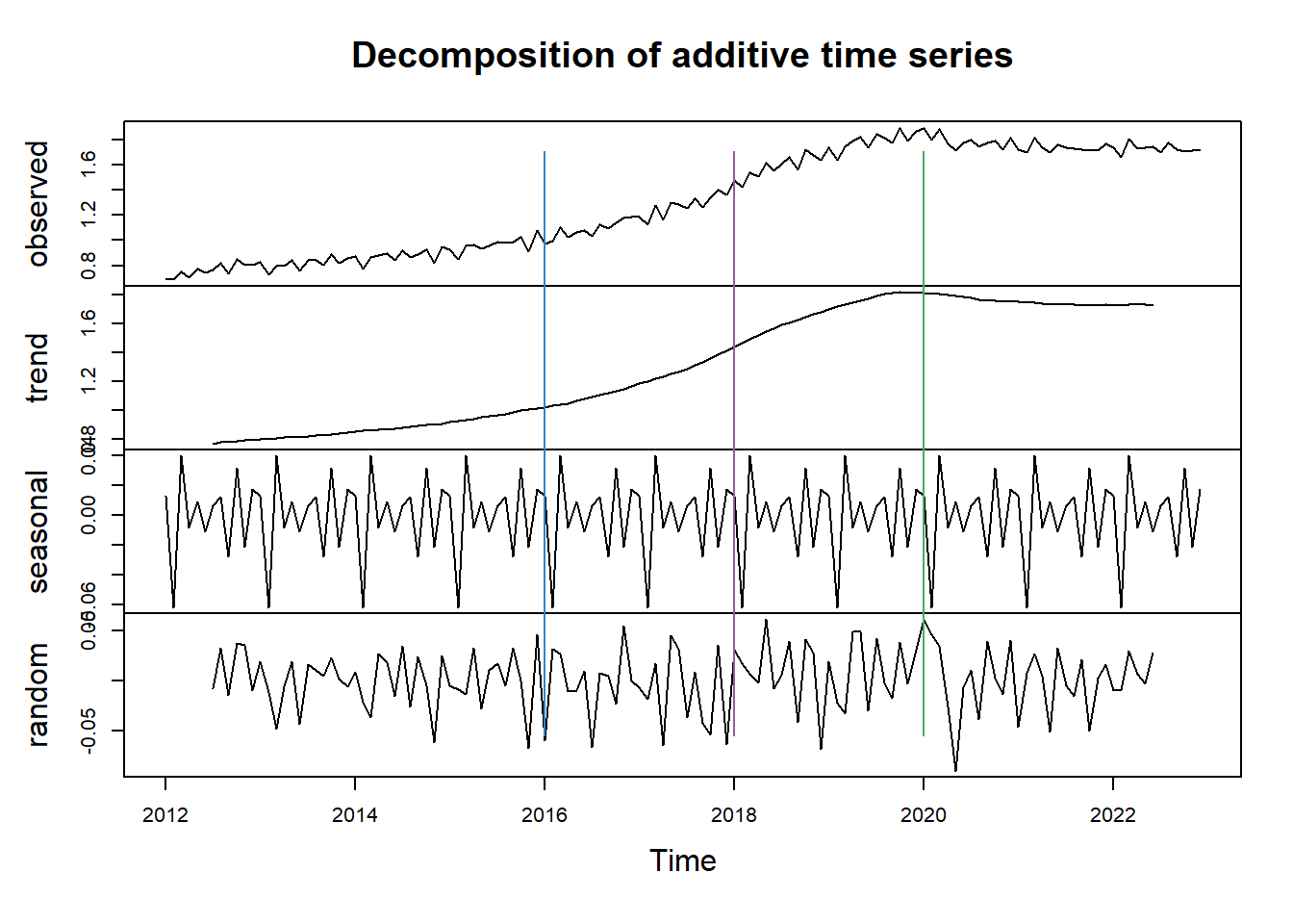
You may also wish to use the decompose() function to break down the time series into its seasonal, trend, and random components. This makes it easier to see the time-series components.
decomposes(bupe_ts): This is the core function in R for decomposing time series data. It breaks down ‘bupe_ts’ time series into the following components:
Trend: The overall, potentially long-term direction of the time series (upward, downward, or stagnant).
Seasonal: Recurring patterns that happen within a fixed period (e.g., spikes each December if you have monthly data).
Random: Irregular, seemingly unpredictable fluctuations remaining after trend and seasonality have been accounted for.
Reveal the Secret Within
# Decompose the series into its seasonal, trend, and random components plot(decompose(bupe_ts)) #add vertical lines for policy change points abline(v =c(2016,8), col="#3086C3") abline(v =c(2018,11),col="#985B9A") abline(v =c(2020,3), col="#42AE65") #add label to vertical line abline(v =c(2016,8), col="#3086C3") abline(v =c(2018,11),col="#985B9A") abline(v =c(2020,3), col="#42AE65")
What to Look for in the Decompositions
Trend
Direction: Is the general movement of the trend upwards, downwards, or mostly level?
The overall trend appears to be slightly increasing over the 2012-2022 period.
Shape: Is it linear (a steady trend line) or curvilinear (indicating the rate of change itself isn’t constant)?
There is some curvature in the trend, suggesting the rate of increase is slowing down over time. This could indicate the dispensation rates have slowed down or stopped increasing.
Seasonal
Strength: Are the peaks and troughs in the seasonality very large in magnitude (strong seasonality) or relatively minor (weak seasonality)?
There is clear seasonality with peaks later in each year.
Regularity: Do the peaks and troughs appear at fixed intervals, or is the pattern less well-defined?
The magnitude of the seasonal peaks seems to be increasing over time. This could indicate higher dispensation rates over time.
Random:
Size: Is this component large in scale compared to the trend and seasonality? This means your data has greater inherent randomness.
The random component appears to be relatively small compared to the trend and seasonality.
Pattern: Can you find any pattern in this residual data, or is it truly unpredictable?
There might be some clustering of values around the trend line in the later years, suggesting potential patterns in the randomness not captured by the seasonal component.
Overall Interpretation:
The bupe_ts series exhibits an increasing trend with clear seasonal peaks in the fall months. The seasonality appears to be strengthening over time, while the random component is relatively small.
Key Points
Visual Analysis:
Decomposition is primarily a visual tool to help you understand the structure of your time series.
Model Assumptions:
Different modeling methods (like ARIMA) have assumptions about the nature of trend, seasonality, and randomness. Your decomposition plots help you choose a suitable approach.
Context is Everything:
Analyze these plots alongside your knowledge of the real-world process that generated your ‘bupe_ts’ data for the most meaningful interpretation.
In an interrupted time-series analysis, you should consider the trend, seasonality, and random graphs around the time periods related to the interruptions. This will usually tell you if an interrupted time-series analysis is appropriate or not. If there isn’t much of a trend before and after the interruption then it may not be necessary.
10.5 Create Intervention Effects
Next, we will specify and add intervention effects for each policy period. The policy period will be based on the following year and month:
DATA 2000 - Jan 2012 to July 2016 (t= 1 to 55)
CARA - July 2016 to October 2018 (t= 56 to 82)
SUPPORT - November 2018 to February 2020 (t= 83 to 98)
COVID-19- March 2020 to December 2022 (t= 99 to 132)
COVID-19 Public Health Emergency Period - March 2020 to May 2020 (t= 99 to 101)
10.5.1 Immediate Change or Effect
In ITS analysis, the immediate variable can be used to assess the immediate impact of the intervention. By including this variable in a time series model (as regressors), you can estimate how the level of the time series changes immediately after the intervention, while controlling for pre-existing trends and patterns.
For the immediate change, you’re creating a series of binary variables to represent the immediate effect of various policy interventions (CARA, SUPPORT, COVID-19, and the short-term COVID-19 stay-at-home order). Each variable is 1 at the time point when the respective policy begins and 0 otherwise.
Reveal the Secret Within
# Create variables representing the immediate effect of each policy# These variables are binary, marking the start of each policy period with 1, otherwise 0# Create a variable for the immediate effect of the CARA policy# It will be 1 at the start of the CARA period (Jul 2016) and 0 otherwiseimmediate_CARA <-as.numeric(as.yearmon(time(bupe_ts)) =="Aug 2016")# Create a variable for the immediate effect of the SUPPORT policy# It will be 1 at the start of the SUPPORT period (Nov 2018) and 0 otherwiseimmediate_SUPPORT <-as.numeric(as.yearmon(time(bupe_ts)) =="Nov 2018")# Create a variable for the immediate effect of the COVID-19 policy# It will be 1 at the start of the COVID-19 period (March 2020) and 0 otherwiseimmediate_COVID19 <-as.numeric(as.yearmon(time(bupe_ts)) =="March 2020")# Create a variable for the immediate effect of the short-term COVID-19 policy (3-month stay-at-home order)# It will be 1 at the start of this short-term period (March 2020) and 0 otherwiseimmediate_COVID19_short_term <-as.numeric(as.yearmon(time(bupe_ts)) =="March 2020")
10.5.2 Step Change or Effect
The “step change” is a way to mark this event in your data. Before the event, the step value is 0; after the event, it’s 1.
This is like drawing a line at the point of the event — one side of the line (before the event) is marked 0, and the other side (after the event) is marked 1.
The step change doesn’t just show an immediate jump or drop; it also helps you see the ongoing effect. For instance, if the rates keep growing steadily after the intervention, that suggests a lasting positive association. This helps you clearly see and measure how things changed from that point onwards, giving you a before-and-after picture of the event’s impact. This is very useful in where you want to understand the effect of decisions or events over time.
For the step change, you’re creating a series of binary variables to represent the step effect of various policy interventions. Each variable is set to 1 for the time period following the start of a respective policy and remains 1 thereafter. These variables include the periods after the introduction of the CARA, SUPPORT policies, COVID-19 period, and the specific 3-month COVID-19 stay-at-home order.
Reveal the Secret Within
# Convert the time component of the bupe_ts time series to Date format# Create variables representing the step effect (change in level) of each policy# These variables are binary, marking the period after the start of each policy with 1, otherwise 0# Create a variable for the step effect post-CARA policystep_CARA <-as.numeric(as.Date(time(bupe_ts)) >=as.Date("2016-08-01", "%Y-%m-%d"))# Create a variable for the step effect post-SUPPORT policy step_SUPPORT <-as.numeric(as.Date(time(bupe_ts)) >=as.Date("2018-11-01", "%Y-%m-%d")) # Create a variable for the step effect post-COVID-19 policy step_COVID19 <-as.numeric(as.Date(time(bupe_ts)) >=as.Date("2020-03-01", "%Y-%m-%d")) # Create a variable for the step effect during the short-term COVID-19 policy period (3-month stay-at-home order) step_COVID19_short_term <-as.numeric(as.Date(time(bupe_ts)) %in%c(as.Date("2020-03-01", "%Y-%m-%d"),as.Date("2020-04-01", "%Y-%m-%d"),as.Date("2020-05-01", "%Y-%m-%d") ))
10.5.3 Ramp Change or Effect
The ramp effect in interrupted time series analysis is used to study a gradual change over time following an intervention, rather than an immediate jump or drop (as in a step change). This gradual change is like a slope or ramp that either increases or decreases steadily after the intervention. In statistical models (like regression models used in time series analysis), this ramp variable can be included to capture and quantify the gradual trend change due to the intervention.
For the ramp effect, you’re creating several variables to represent the ramp effect for different policy periods. These variables capture the gradual change over time during and after each policy period, reflecting an increasing trend over the duration of each policy or the ongoing trends from the start of each respective policy period through to the end of the time series data.
Reveal the Secret Within
# Create variables representing the ramp effect (gradual change over time) for each policy# These variables capture the trend over time during and after each policy period# Create a ramp variable for the CARA policy periodramp_CARA <-append(rep(0, length(bupe_ts[as.Date(time(bupe_ts)) <=as.Date("2016-08-01", "%Y-%m-%d")])), seq(1, length(bupe_ts[as.Date(time(bupe_ts)) >as.Date("2016-08-01", "%Y-%m-%d") &as.Date(time(bupe_ts)) <=as.Date("2022-12-01", "%Y-%m-%d")]), 1))# Create a ramp variable for the SUPPORT policy periodramp_SUPPORT <-append(rep(0, length(bupe_ts[as.Date(time(bupe_ts)) <=as.Date("2018-11-01", "%Y-%m-%d")])), seq(1, length(bupe_ts[as.Date(time(bupe_ts)) >as.Date("2018-11-01", "%Y-%m-%d") &as.Date(time(bupe_ts)) <=as.Date("2022-12-01", "%Y-%m-%d")]), 1))# Create a ramp variable for the COVID-19 policy periodramp_COVID19 <-append(rep(0, length(bupe_ts[as.Date(time(bupe_ts)) <=as.Date("2020-02-01", "%Y-%m-%d")])), seq(1, length(bupe_ts[as.Date(time(bupe_ts)) >as.Date("2020-02-01", "%Y-%m-%d") &as.Date(time(bupe_ts)) <=as.Date("2022-12-01", "%Y-%m-%d")]), 1))
11 Create a Time Series Tibble
11.1 Build a Predictor Matrix
Immediate Impact:
If there is an immediate shift in the time-series after the initiation of an intervention, the immediate effects would measure this.
We will drop immediate effects from the list of predictors, since it is obvious graphically that there is no immediate level shift.
Lasting Level Shifts (Step Effect):
The step effect aims to measure a permanent shift in the time-series after an intervention.
Although the time-series seems to change after each policy implementation, there also seems to be a gradual change before and after the policies that would may be captured in the ramping effect.
The exception is the short period following the COVID-19 Public Health Emergency order in March 2020. The random component of the decomposed series seems to suggest a significant change in that period that is not completely accounted by the trend or seasonal components. This may have resulted in the on-going ramp effect after this period.
Ongoing Trends (Ramp Effect):
The ramp effect captures the gradual, continuous changes in the time series following the intervention. This effect is key for understanding the long-term trend or trajectory of the time series as a result of the intervention.
Reveal the Secret Within
# Create a matrix of covariates to use in the ARIMA model or other models combining different effect variables# 'final_predictors' will include the ramp effect variables for DATA 2000, CARA, SUPPORT, and COVID-19, as well as the step effect variable for the short-term COVID-19 periodfinal_predictors <- tibble::tibble(t =seq.int(from =1, to =length(bupe_ts)),ramp_CARA = ramp_CARA,ramp_SUPPORT = ramp_SUPPORT,ramp_COVID19 = ramp_COVID19,step_COVID19_short_term = step_COVID19_short_term ) #clean up environmentrm(immediate_CARA, immediate_COVID19, immediate_COVID19_short_term,immediate_SUPPORT, step_CARA, step_SUPPORT, step_COVID19, step_COVID19_short_term, ramp_CARA, ramp_SUPPORT, ramp_COVID19)
With the predictors and rates, we can combine them all together into a single tibble to use more easily with other R packages for modeling.
Reveal the Secret Within
final_data <-tibble(month_year =seq.Date(from =as.Date("2012-01-01"), to =as.Date("2022-12-01"),by ="months"),t =seq.int(from =1, to =length(bupe_ts), by =1),outcome =as.numeric(bupe_ts) ) %>% dplyr::inner_join( final_predictors,by =c("t") )
11.2 Check for Auto-Correlation
Remember in a time series analysis, we are assuming that the time series has autocorrelation and will thus need a more advanced statistical model to measure those correlations correctly. Below are a few of the options we can use to check and see if we need a simple linear regression model or a more advanced statistical model (or other adjustments).
Measures the correlation between a time series and its lagged values. In simpler terms, it indicates how much the data at a given point in time is related to its own past values.
Reveal the Secret Within
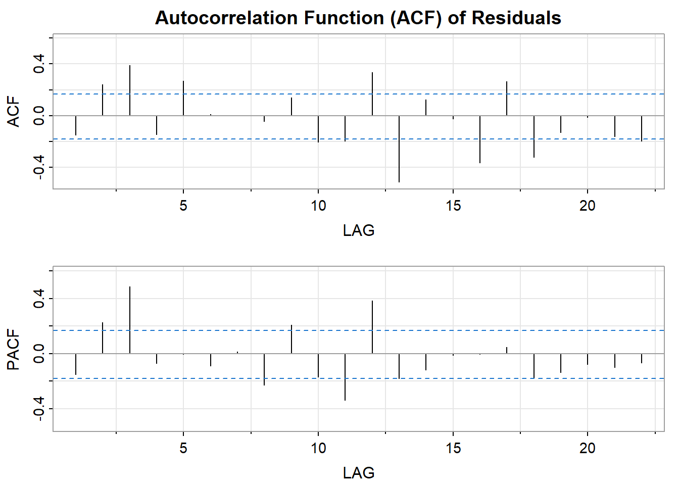
# View ACF/PACF plots of buprenorphine series data acf_bupe_ts <- astsa::acf2(bupe_ts, main=paste0("ACF of Series"))
Do the bars decline rapidly near the beginning or more gradually across lags?
The ACF plot shows a slow decay over time.
There is a significant spice during the first lag in the PACF plot.
There are regular spikes at each 12 lag and they seem to be weaking over a long lag.
11.2.0.2 Statistical Tests for Autocorrelation
Fit a linear regression model to your data.
Reveal the Secret Within
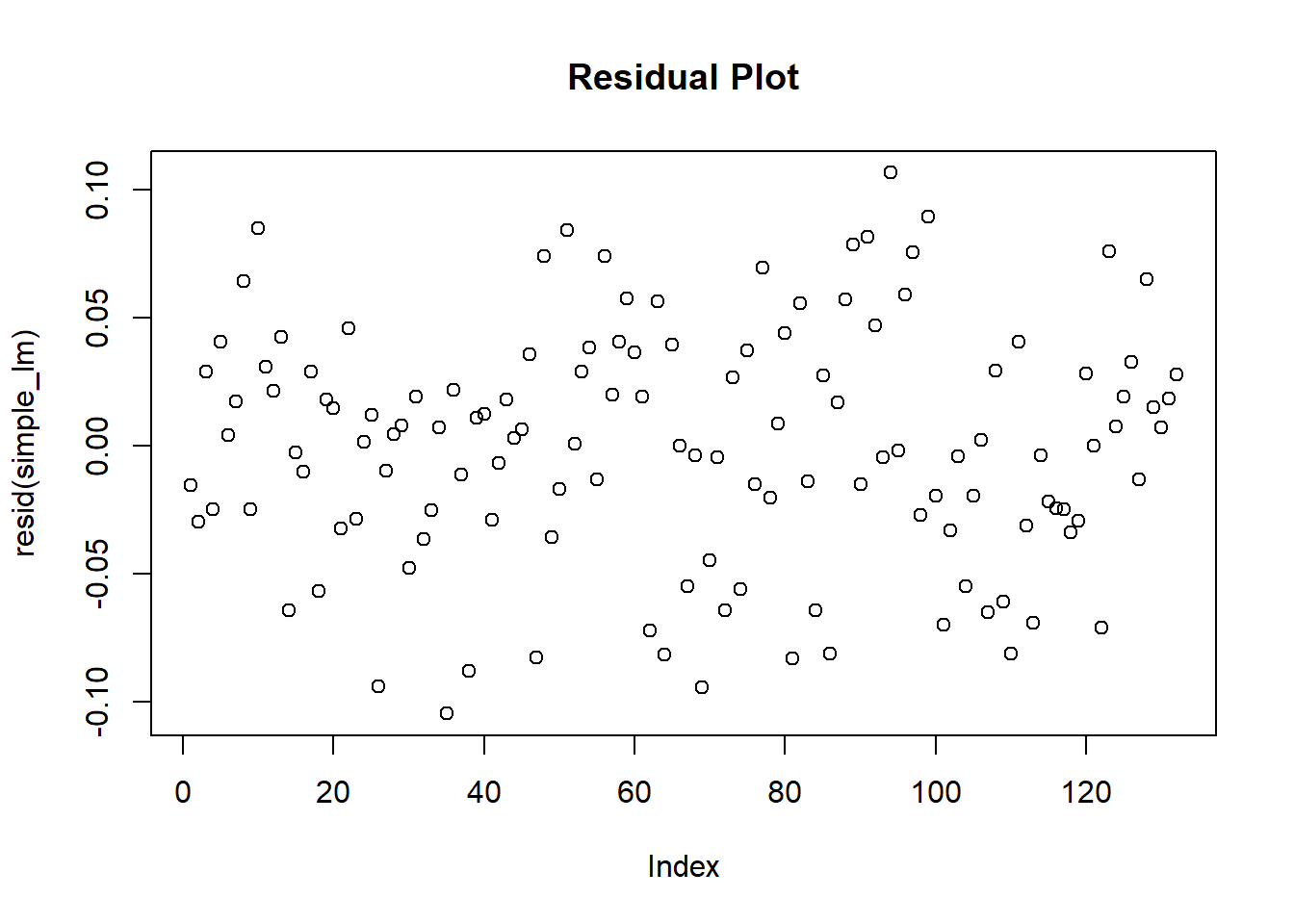
# Simple Linear Regression Model simple_lm <-lm(outcome ~ t + ramp_CARA + ramp_SUPPORT + ramp_COVID19 + step_COVID19_short_term, data = final_data) # View Model Summary summary(simple_lm) # Use Summary for more comprehensive output
Call:
lm(formula = outcome ~ t + ramp_CARA + ramp_SUPPORT + ramp_COVID19 +
    step_COVID19_short_term, data = final_data)

Residuals:
      Min        1Q    Median        3Q       Max
-0.104593 -0.028787  0.001978  0.029074  0.106652

Coefficients:
                          Estimate Std. Error t value             Pr(>|t|)
(Intercept)              0.7050296  0.0121676  57.943 < 0.0000000000000002 ***
t                        0.0062137  0.0003371  18.433 < 0.0000000000000002 ***
ramp_CARA                0.0173413  0.0009289  18.669 < 0.0000000000000002 ***
ramp_SUPPORT            -0.0146807  0.0019434  -7.554     0.00000000000751 ***
ramp_COVID19            -0.0127034  0.0019974  -6.360     0.00000000339626 ***
step_COVID19_short_term -0.0259620  0.0300872  -0.863                 0.39
---
Signif. codes:  0 '***' 0.001 '**' 0.01 '*' 0.05 '.' 0.1 ' ' 1

Residual standard error: 0.04688 on 126 degrees of freedom
Multiple R-squared:  0.9874,    Adjusted R-squared:  0.9869
F-statistic:  1969 on 5 and 126 DF,  p-value: < 0.00000000000000022
A formal statistical test to detect if there’s significant autocorrelation in the residuals.
Null Hypothesis:
H0: The data are independently distributed (i.e. the correlations in the population from which the sample is taken are 0, so that any observed correlations in the data result from randomness of the sampling process).
    Durbin-Watson test

data:  final_data$outcome ~ final_data$t + final_data$ramp_CARA + final_data$ramp_SUPPORT +     final_data$ramp_COVID19 + final_data$step_COVID19_short_term
DW = 2.2971, p-value = 0.9034
alternative hypothesis: true autocorrelation is greater than 0
Ljung-Box Test (Box.test):
The Ljung-Box test checks for autocorrelation in the residuals of a time series model. Autocorrelation here means that the residuals (errors) of the model are correlated with each other at different lags.
Null Hypothesis:
H0: The data are independently distributed (i.e. the correlations in the population from which the sample is taken are 0, so that any observed correlations in the data result from randomness of the sampling process).
Reveal the Secret Within
## Box-Ljung test Box.test(simple_lm$residuals, lag =24, type ="Ljung-Box")
Since the residuals are correlated from a simple linear model, we will now proceed with using an AR(k) model using the auto.arima() function from the forecast package in R.
By using the auto.arima() function from the forecast package in R, you can automatically select the best ARIMA model while considering these covariates. This function examines various combinations of ARIMA models and chooses the one that best fits your data, taking into account the immediate, step, and ramp effects. This approach is powerful for analyzing time series data, as it provides a comprehensive view of how different types of interventions or events impact the data over time.
12.1 Using auto.arima() with expanded search parameters
This code uses the auto.arima function to automatically fit an ARIMA (Autoregressive Integrated Moving Average) model to the buprenorphine time series data (bupe_ts) and the final_predictors dataset we created earlier.
Reveal the Secret Within
# Fit an ARIMA model to the bupe_ts time series data using the 'auto.arima' functionmodel <- forecast::auto.arima(bupe_ts, seasonal=TRUE, # Consider seasonal components in the modelxreg=as.matrix(final_predictors), # Include the matrix of covariates (ramp effects) as external regressorsstepwise = F, # Disable stepwise algorithm for model selectionapproximation = F, # Disable approximation for more accurate model fittingtrace = F, # Enable detailed output of the model fitting processmax.p =30, # Set the maximum order for the AR componentmax.q =30, # Set the maximum order for the MA componentmax.d =30) # Set the maximum order for the differencing component
Assigning the Model:
model <-:
This line is where the magic happens. auto.arima is a powerful function from the forecast package. It will try different combinations of ARIMA parameters (p, d, q) to find the best-fitting model based on a criterion like AICc (a measure of model goodness-of-fit with a penalty for complexity).
The result of the model fitting is stored in a variable named model.
The Time Series Data:
bupe_ts: This is the time series data that the ARIMA model will be fitted to. In this context, bupe_ts represents a time series of the log-transformed sex-age adjusted buprenorphine prescription rates for all prescribers.
Seasonality:
seasonal=TRUE: Indicates that the auto.arima function should consider seasonal ARIMA models. This suggests there might be recurring patterns related to seasons (e.g., increased buprenorphine dispensation during certain months of the year).
External Regressors:
This incorporates your final_predictors matrix as external regressors.
External regressors are like “helper variables” that can improve the model’s predictive power. These are the covariates or predictors explaining the time-series. In this case, they are the ramp effects of interest and the step effect of the COVID-19 public health emergency period. By including these covariates, the model is designed to capture both immediate and long-term effects of policies, providing a richer understanding of how these interventions have impacted the time series data.
Model Selection Parameters:
stepwise = F: Turns off a stepwise search algorithm for model selection. This means the function will try a wider range of p, d, q combinations.
approximation = F: Disables an approximation that sometimes speeds up the model fitting, but at the cost of potentially less accurate results.
trace = F: Gives you verbose output during the model selection process, so you can track how the auto.arima function is iterating.
Model Complexity Limits:
max.p = 30, max.q = 30, max.d = 30: These arguments set the maximum order for the AR (p), MA (q), and differencing (d) components of the ARIMA model. Setting these to 30 allows for a wide range of models to be considered, but it also increases computational demand.
max.p = 30: The maximum number of autoregressive terms.
max.q = 30: The maximum number of moving average terms.
max.d = 30: The maximum number of differences used to make the series stationary.
The auto.arima function automates a lot, but remember to check the diagnostics plots generated from your final model. It’s a good idea to verify that the model’s residuals don’t have autocorrelation and meet necessary assumptions.
Using the final ARIMA selected, the R code below uses the arima() function to fit that model into an arima object (easier for R to use).
12.2 Model Estimates
Below is the R code and its output pertain to the summary and confidence intervals of the ARIMA model found previously for our interrupted time series model.
Reveal the Secret Within
summary(arima_model)
Call:
arima(x = bupe_ts, order = c(arma_orders[1], arma_orders[2], arma_orders[3]),
    seasonal = list(order = c(arma_orders[4], arma_orders[5], arma_orders[6]),
        period = arma_orders[7]), xreg = as.matrix(final_predictors), method = "CSS-ML")

Coefficients:
         ar1     ar2     ar3      ar4    sma1  intercept       t  ramp_CARA
      0.0131  0.3861  0.3834  -0.2015  0.5005     0.7007  0.0065     0.0160
s.e.  0.0934  0.0785  0.0848   0.0922  0.0842     0.0256  0.0007     0.0019
      ramp_SUPPORT  ramp_COVID19  step_COVID19_short_term
           -0.0109       -0.0159                  -0.0490
s.e.        0.0034        0.0032                   0.0167

sigma^2 estimated as 0.001174:  log likelihood = 255.88,  aic = -487.76

Training set error measures:
                         ME       RMSE        MAE         MPE     MAPE
Training set -0.00006128062 0.03426185 0.02680637 -0.09350372 2.197146
                  MASE         ACF1
Training set 0.4585076 -0.002211555
Regression with ARIMA(4,0,0)(0,0,1)[12] errors
Regression: You’ve included external predictors.
ARIMA(4,0,0): The core ARIMA component has:
AR(4): An autoregressive term of order 4 (current value depends on the past 4 values).
0 for ‘d’: No differencing.
MA(0): No moving average component.
(0,0,1)[12] A seasonal moving average (SMA) term of order 1 with a period of 12 (for monthly data).
Coefficients:
ar1, ar2, ar3, ar4: Coefficients for the autoregressive components, expressing the effect of past buprenorphine dispensation rates. These are the coefficients for the four autoregressive terms. They are relatively small, with ar1 being positive and quite small (0.0131), ar2 and ar3 being larger and positive (0.3861 and 0.3834 respectively), and ar4 being negative (-0.2015). This suggests a complex pattern where the past values have a fluctuating influence on the current value.
sma1: The coefficient for the seasonal moving average term (smoothing effects from values 12 months prior). The coefficient for the seasonal moving average at lag 12 is positive (0.5005), indicating a strong seasonal effect in the past data that influences the current value.
intercept: The baseline average level of buprenorphine rates when variables are zero. The model includes an intercept (0.7007), which is the expected mean level of the series when all other factors are zero.
t: Represents a linear time trend. The coefficient for time trend (0.0065) is very small, suggesting a slight increasing or decreasing trend in the series.
ramp_CARA and ramp_SUPPORT: These coefficients (0.0160 and -0.0109 respectively) represent the trend or sustained effects associated with the post-implementation of the CARA and SUPPORT policy. Their magnitude shows the estimated change in buprenorphine dispensation rates per unit change in each of those predictors.
step_COVID19_short-term, ramp_COVID19: These coefficients (-0.0490 and -0.0159) represent the short-term step change and a linear ramp effect associated with COVID-19.
s.e.: Standard errors of the coefficients, signifying the estimation uncertainty.
Model Fit Statistics:
sigma^2: The estimated variance of the residuals is very low (0.001281), indicating a good fit of the model to the data.
log likelihood: The log likelihood value is quite high (255.88), which is good as it means the observed data is very likely under the fitted model
Error Measures:
These offer various ways to gauge how well your model performed on the data it was trained (modeled/fitted) on:
ME: Mean Error (should be close to zero)
RMSE: Root Mean Squared Error (smaller is better)
MAE: Mean Absolute Error (smaller is better)
MPE: Mean Percentage Error
MAPE: Mean Absolute Percentage Error
MASE: Mean Absolute Scaled Error
ACF1: Autocorrelation at lag 1 (ideally close to zero, your model seems good here)
The RMSE and MAE are very low, indicating good predictive accuracy.
The MPE and MAPE are measures of forecast bias and accuracy, respectively, and both are quite low, which is favorable.
MASE compares the model’s forecast error to the naive model; it is also low. ACF1 is near zero, suggesting little to no autocorrelation in the residuals, which is desirable.
12.2.1 Confidence Intervals of Coefficients
This function provides the confidence intervals for the model’s coefficients.
For each parameter, it gives a range (2.5 % and 97.5 % columns) within which we can be 95% confident that the true value of the coefficient lies.
12.2.3 Test Linear Hypothesis and Generate Policy Effects
This code aims to test specific hypotheses about the policy-related coefficients (and their linear combinations) in your fitted ARIMA model, potentially examining how changing a combination of policies would impact buprenorphine prescription rates.
linearHypothesis(): A function (from the car package) tests a statistical hypothesis regarding linear combinations of the coefficients in your ARIMA model (model).
Each test specifies a hypothesis:
CARA Ramp:
Tests if the effect of both the time trend (t) and ramp_CARA can be considered negligible (equal to zero).
SUPPORT Ramp:
Tests if the combined effect of t, ramp_CARA, and ramp_SUPPORT equals zero.
COVID-19 Ramp:
Tests if the combined effect of t, ramp_CARA, ramp_SUPPORT, and ramp_COVID19 equals zero.
Reveal the Secret Within
# Test hypothesis and effect of each policy hypothesis_result <- dplyr::bind_rows(# CARA Ramp Effecttidy(linearHypothesis(arima_model, c("t + ramp_CARA = 0"))),# SUPPORT Ramp Effecttidy(linearHypothesis( arima_model, c("t + ramp_CARA + ramp_SUPPORT = 0") )),# COVID-19 Ramp Effecttidy(linearHypothesis( arima_model, c("t + ramp_CARA + ramp_SUPPORT + ramp_COVID19 = 0") )) ) %>% janitor::clean_names() %>% dplyr::mutate(exp_estimate =100* (exp(estimate) -1)) hypothesis_result
All three hypothesis tests are statistically significant, as indicated by the very small p-values. This means we reject the null hypotheses that the specified policy combinations have zero effect on buprenorphine dispensation rates.
Specific Results
CARA Ramp Hypothesis:
The test supports that the combined effect of t (time trend) and ramp_CARA is likely not equal to zero.
The positive exp_estimate (2.27%) suggests that these factors collectively is associated with an increase in buprenorphine dispensation rates by approximately 2.27%.
SUPPORT Ramp Hypothesis:
The test suggests that the combined effect of t, ramp_CARA, and ramp_SUPPORT is also unlikely to be zero.
The exp_estimate of 1.16% implies an associated increase in buprenorphine dispensation rates.
COVID-19 Ramp Hypothesis:
The combined effect of t, ramp_CARA, ramp_SUPPORT, and ramp_COVID19 is likely not zero.
Interestingly, the exp_estimate is negative (-0.431%), suggesting that this combined effect might be very slightly associated with a decrease in buprenorphine dispensation rates.
Important Considerations
Correlation vs. Causation:
Although statistically significant, these tests alone don’t definitively prove that these policies were solely responsible for the changes in buprenorphine rates.
You need to carefully consider real-world events and factors alongside these analyses.
Magnitude of Effects:
The percentage changes (while statistically significant) appear relatively small in magnitude.
Consider whether these have practical importance alongside your statistical evaluations.
Other Covariates:
If your model contains other factors alongside these policy-related variables, these will influence how you interpret the results.
12.3 Model Diagnostics
In the context of time series forecasting and ARIMA models, residuals are the differences between the observed values of your time series and the values predicted by the model. Essentially, they are the part of the data that the model couldn’t explain.
Analyzing the residuals of a model is crucial. It helps to assess whether the model fits the data well. If the residuals show no clear patterns and resemble white noise, it suggests that the model has captured most of the information in the data. However, if there are patterns or trends in the residuals, it implies that there is still some information in the data that the model hasn’t captured.
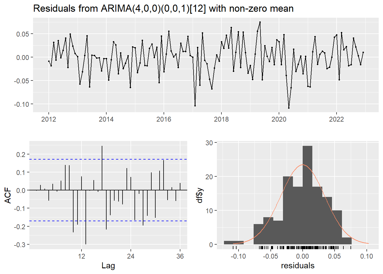
12.3.1 Check Residuals with checkresiduals()
The checkresiduals() is a function from the forecast package in R. It’s used to perform a diagnostic check on the residuals of a time series model.
What It Does:
Residual Plot: It plots the residuals, allowing you to visually inspect if there’s any obvious pattern or trend. Ideally, the residuals should appear as a random scatter, indicating that they are just noise.
ACF Plot: The function also includes an Autocorrelation Function (ACF) plot of the residuals. This plot helps to check for autocorrelation; if the residuals are uncorrelated, most of the autocorrelations should be within the blue dashed lines, which represent a 95% confidence interval.
Statistical Tests: It typically runs a Ljung-Box test or similar to quantitatively assess whether there is significant autocorrelation in the residuals. A high p-value (typically above 0.05) suggests that the residuals are independent, which is a good sign for the model.
Using checkresiduals(arima_model), you’re essentially performing a health check on your ARIMA model. This function will show you if the model is leaving out any significant information in the residuals. It’s a crucial step in model validation, ensuring that your forecasts are as accurate and reliable as possible.
Reveal the Secret Within
# check residuals of ARIMA Modelcheckresiduals(arima_model)
    Ljung-Box test

data:  Residuals from ARIMA(4,0,0)(0,0,1)[12] with non-zero mean
Q* = 59.84, df = 19, p-value = 0.000004103

Model df: 5.   Total lags used: 24
From the checkresiduals(arima_model) , the following results are interpreted as such:
The Null Hypothesis is Rejected: The very small p-value (p < 0.0001) means that it’s extremely unlikely to obtain this Q* statistic if the residuals were truly random. Therefore, we reject the null hypothesis that the residuals are independently distributed.
Autocorrelation Exists: This result indicates that autocorrelation is present in the residuals of your ARIMA model. Autocorrelation means that there are patterns remaining in the errors, suggesting your model hasn’t fully captured all the predictable information in the time series.
Details from the Test
Q Statistic:* 59.84 – This measures the overall degree of autocorrelation throughout the lags examined.
Degrees of Freedom (df): 19 – This depends on the number of lags tested and parameters in the ARIMA model.
Model df: 5 – The degrees of freedom associated with the parameters estimated in your ARIMA(4,0,0)(0,0,1)[12] model.
Total Lags Used: 24 – The test evaluated autocorrelation across 24 lags.
Next Steps
Model Revision:
Given the presence of autocorrelation, your ARIMA model likely needs adjustment. You might consider experimenting with different ARIMA orders or including additional variables that could explain the patterns in the residuals.
Investigate Causes:
Try to identify the causes of the autocorrelation (e.g., omitted variables, potential structural changes, non-linear relationships).
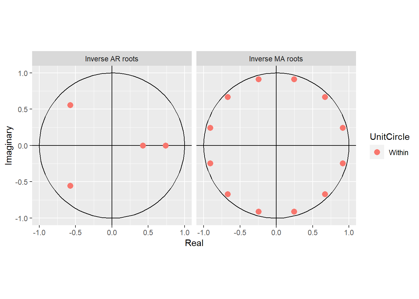
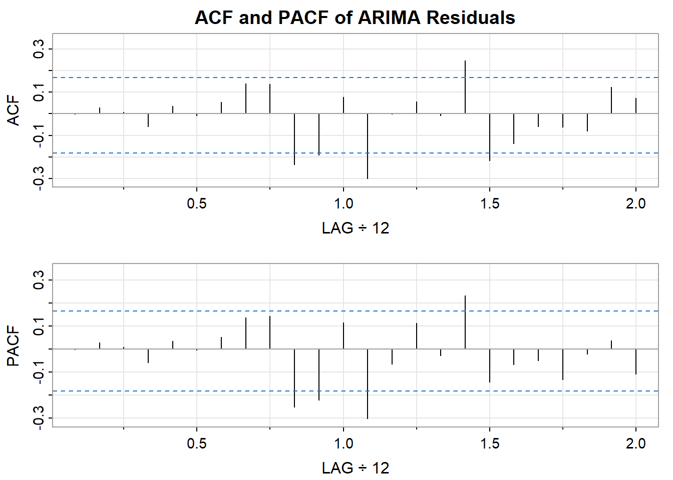
12.3.2 Check ACF, PACF, and Residuals
Although the model still has some autocorrelation remaining, which means there are other factors remaining that may still explain the time series, you should check the residuals of the model for auto correlation. The residuals should not have any autocorrelation and should represent a stationary time series for a properly fitted ARIMA model.
Reveal the Secret Within
# check whether AR terms are within the unit circleautoplot(arima_model)
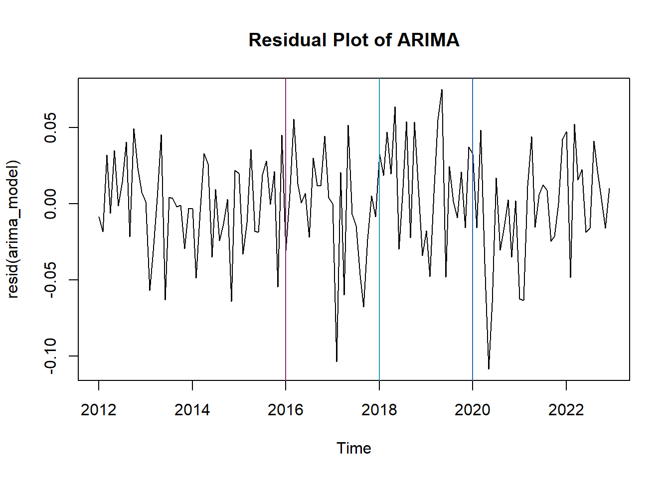
Reveal the Secret Within
# plot of residiuals from ARIMA modelplot(resid(arima_model)) +title(main ="Residual Plot of ARIMA")
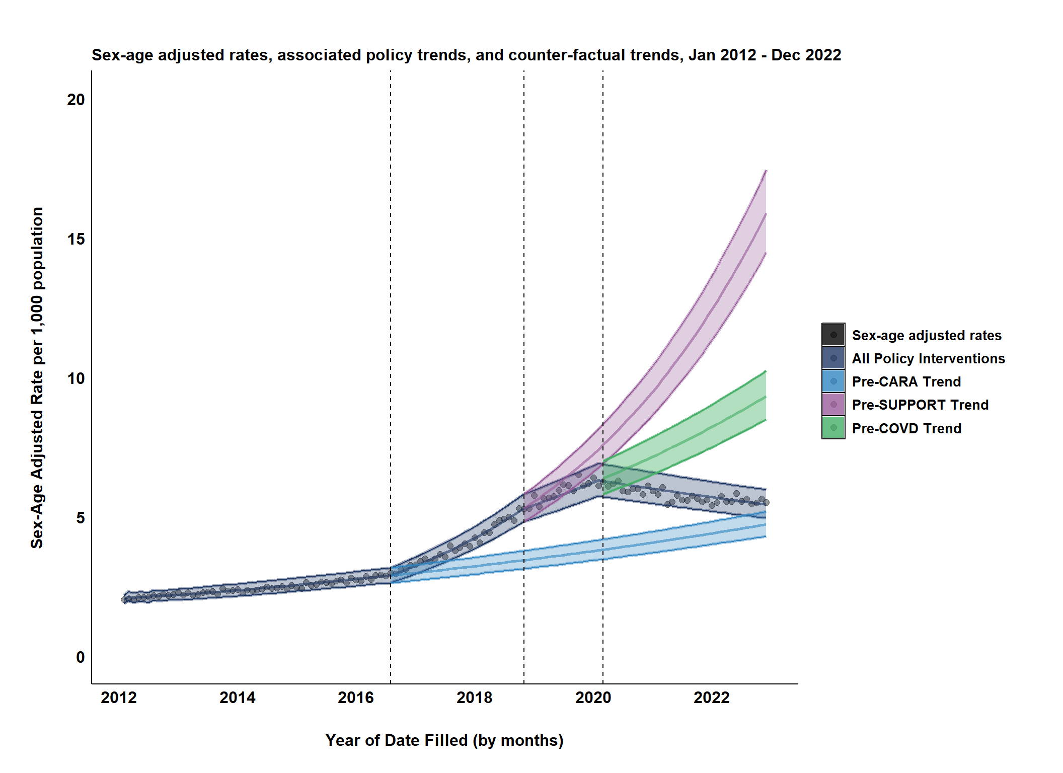
The primary aim of this code is to create forecasts of buprenorphine dispensation rates assuming your various policy variables (ramp_CARA, etc.) had been set to zero. This serves as a counterfactual scenario or baseline to help isolate the policies’ potential impact.
This approach provides a way to estimate the counter-factual scenario, essentially allowing you to compare the actual post-intervention data with what the model predicts would have happened without the intervention. This comparison can be insightful for understanding the impact of the intervention.
Why Forecasting Matters
Extrapolating the Baseline: The predicted counterfactual trend is not static. Forecasting it forward tells us where the buprenorphine levels might have settled in the absence of the policy. This is important for comparing outcomes over time.
Anticipating Potential Outcomes: If we assume the historical trends or patterns would have mostly continued, the counterfactual forecasts give us a guideline for what outcomes to expect without the policy.
Quantifiable Differences: The gap between the actual data and the forecasted counterfactual offers a numerical estimate of the policy’s effect at specific points in time into the future.
Understanding the “What If”: Counterfactuals help answer the question “What would have likely happened if a policy hadn’t been implemented?” In ITS, plotting the observed outcome (buprenorphine dispensation rates) against the predicted counterfactual provides a visual intuition of the policy’s potential effect.
Trend Comprehension: Comparing pre- and post-intervention trends visually shows whether a policy led to changes in the level and trend of the buprenorphine dispensation rates. Statistical tests offer quantifiable measures but a plot communicates this impact quickly.
Identifying Deviations: Were there increases/decreases in buprenorphine rates following the policy introduction that can’t be explained by the extrapolated continuation of the pre-intervention trend? An visual makes these deviations much clearer.
Limitations to Consider
Assumptions: Interrupted time series methods (and any forecasts) are heavily reliant on the assumption that the trends would have continued. External events unrelated to the policies under study can skew results.
Interpretation: Counterfactuals are a helpful tool, but cannot definitively prove causation. It’s essential to assess your policy effects together with expert domain knowledge about real-world events that could be involved.
13.1 Create Counter-factual Predictor Datasets
1. Data Preparation
pre_cara_predictors <- ...
Creates a copy of your final_predictors data.
Uses dplyr::mutate to overwrite the ramp_CARA, ramp_SUPPORT, and COVID-related policy variables, setting them to zero. This isolates the effect of removing CARA policies.
pre_support_predictors <- ...
Same concept, but sets only ramp_SUPPORT and COVID-related policy variables to zero, isolating the SUPPORT policy impact.
pre_covid19_predictors <- ...
Prepares the dataset to isolate the COVID-19 related policy impacts.
Reveal the Secret Within
# Pre-CARA Scenario: Create a copy of your predictors and set CARA and COVID policies to zeropre_cara_predictors <- final_predictors %>% dplyr::mutate(ramp_CARA =0, # Set CARA ramp effect to zeroramp_SUPPORT =0, # Set SUPPORT ramp effect to zeroramp_COVID19 =0, # Set COVID-19 ramp effect to zerostep_COVID19_short_term =0# Set COVID-19 short-term step effect to zero )# Pre-SUPPORT Scenario: Similar, but focus on removing SUPPORT policiespre_support_predictors <- final_predictors %>% dplyr::mutate(ramp_SUPPORT =0, ramp_COVID19 =0, step_COVID19_short_term =0 )# Pre-COVID Scenario: Isolate the removal of COVID-related policiespre_covid19_predictors <- final_predictors %>% dplyr::mutate(ramp_COVID19 =0,step_COVID19_short_term =0 )
13.2 Forecast Generation: Calculate Predictions Under Each Scenario
forecast::forecast(...)
forecast::forecast() : Generates forecasts from your fitted ARIMA model (model).
xreg = ... : Uses the modified pre_cara_predictors , pre_support_predictors, and pre_covid_predictors predictors that isolate and remove the effects of CARA, SUPPORT, and/or COVID policies.
level = c(0.95): Requests 95% confidence intervals for the predictions.
h = length(bupe_ts): Specifies how many data points (equal to the length of your existing buprenorphine time series) should be forecast ahead.
Reveal the Secret Within
#--- Forecast Generation: Calculate Predictions Under Each Scenario ---## Pre-CARA Forecast: Generate forecasts assuming CARA policies were absentpre_cara_forecast <- forecast::forecast(model,xreg =as.matrix(pre_cara_predictors),level =c(0.95), # Include 95% confidence intervalsh =length(bupe_ts)) # Forecast for same length as original data# Pre-SUPPORT Forecast: Identical concept, removing SUPPORT policiespre_support_forecast <- forecast::forecast(model,xreg =as.matrix(pre_support_predictors),level =c(0.95), h =length(bupe_ts))# Pre-COVID Forecast: Forecast under the hypothetical removal of COVID policiespre_covid_forecast <- forecast::forecast(model,xreg =as.matrix(pre_covid19_predictors),level =c(0.95), h =length(bupe_ts))# All Effects Forecast: Forecast under the hypothetical removal of COVID policiesall_data_forecast <- forecast::forecast( model,xreg =as.matrix( final_predictors %>% dplyr::mutate(step_COVID19_short_term =0) ),level =c(0.95),h =length(bupe_ts))
13.3 Create Counter Factual Data
This R code snippet is performing a counterfactual analysis using time series forecasting. It’s designed to estimate what the forecasted values of a target variable (perhaps prescription rates) might have been if certain policies had not been implemented. This is done by setting the policy-related predictors to zero and then generating forecasts based on the modified predictors.
Reveal the Secret Within
# --- Create Structured Data Frame for Visualization and Analysis --- #policy_forecasts <- dplyr::bind_cols(month_year = bupe_rates$month_year, # Preserve the time reference# Include counterfactual trend components (mean forecasts & confidence intervals)pre_cara_trend = pre_cara_forecast$mean,pre_cara_trend_lower95 = pre_cara_forecast$lower[,1],pre_cara_trend_upper95 = pre_cara_forecast$upper[,1],pre_support_trend = pre_support_forecast$mean,pre_support_trend_lower95 = pre_support_forecast$lower[,1],pre_support_trend_upper95 = pre_support_forecast$upper[,1],pre_covid_trend = pre_covid_forecast$mean,pre_covid_trend_lower95 = pre_covid_forecast$lower[,1],pre_covid_trend_upper95 = pre_covid_forecast$upper[,1]) %>%# Ensure conversion to tidy data frame (tibble) tibble::as_tibble() %>%# Clean up column names janitor::clean_names() %>% dplyr::mutate(actual = bupe_rates$prescription_rate, # Add actual buprenorphine rate datafitted = model$fitted, # Include ARIMA model's fitted valuestrend = all_data_forecast$mean, # Include ARIMA model's trend effecttrend_lower95 = all_data_forecast$lower[,1] , # Include ARIMA model's lower 95% trend effecttrend_upper95 = all_data_forecast$upper[,1], # Include ARIMA model's lower 95% trend effect ) %>%# Exponeniate log-rates back to original values dplyr::mutate(across(pre_cara_trend:trend_upper95, exp)) %>%# set trends pre-policies to missing dplyr::mutate(pre_cara_trend =ifelse( month_year < cara_date, NA_real_,pre_cara_trend),pre_support_trend =ifelse( month_year < support_date, NA_real_,pre_support_trend),pre_covid_trend =ifelse( month_year < covid19_date, NA_real_,pre_covid_trend),pre_cara_trend_lower95 =ifelse( month_year < cara_date, NA_real_,pre_cara_trend_lower95),pre_support_trend_lower95 =ifelse( month_year < support_date, NA_real_,pre_support_trend_lower95),pre_covid_trend_lower95 =ifelse( month_year < covid19_date, NA_real_,pre_covid_trend_lower95),pre_cara_trend_upper95 =ifelse( month_year < cara_date, NA_real_,pre_cara_trend_upper95),pre_support_trend_upper95 =ifelse( month_year < support_date, NA_real_,pre_support_trend_upper95),pre_covid_trend_upper95 =ifelse( month_year < covid19_date, NA_real_,pre_covid_trend_upper95) )
13.4 Visualizing the Counter Factual Trends
Reveal the Secret Within
# ---- Data Setup ----# Color palette definitionsdata_colors <-c("black", "#203864", "#3086C3", "#985B9A", "#42AE65")# Labels for descriptive legenddata_labels <-c("Sex-age adjusted rates","All Policy Interventions","Pre-CARA Trend","Pre-SUPPORT Trend","Pre-COVD Trend")# ---- Plotting ----policy_plot <-ggplot(policy_forecasts,aes(x = month_year))# ---- Observed sex-age adjusted rates ----policy_plot <- policy_plot +geom_point(aes(y = fitted, group =1L, color = data_labels[1], fill = data_labels[1]),size =2,alpha =0.4 )# ---- Modeled trend - All policy interventions ----# Increased transparency to improve visual reading# Added linetype specification for visual distinctionpolicy_plot <- policy_plot +geom_line(aes(y = trend, group =1L, color = data_labels[2]),size =1,alpha =0.6,linetype =1 ) +# add 95% confidence bands for trends from the model geom_line(aes(y = trend_lower95, group =1L, color = data_labels[2]),size =1.2,alpha =0.4,linetype =1 ) +geom_line(aes(y = trend_upper95, group =1L, color = data_labels[2]),size =1.2,alpha =0.4,linetype =1 ) +geom_ribbon(aes(ymin = trend_lower95, ymax = trend_upper95, group =1L, color = data_labels[2],fill = data_labels[2]),alpha =0.3# Low alpha for a subtle fill effect )# ---- Pre-CARA Trend Forecasts (assuming DATA 2000 only) ----policy_plot <- policy_plot +# pre-CARA Forecast geom_line(aes(y = pre_cara_trend, group =1L, color = data_labels[3]),size =1,alpha =0.6,linetype =1 ) +geom_line(aes(y = pre_cara_trend_lower95, group =1L, color = data_labels[3]),size =1.2,alpha =0.4,linetype =1 ) +geom_line(aes(y = pre_cara_trend_upper95, group =1L, color = data_labels[3]),size =1.2,alpha =0.4,linetype =1 ) +geom_ribbon(aes(ymin = pre_cara_trend_lower95, ymax = pre_cara_trend_upper95, group =1L, fill= data_labels[3],color = data_labels[3]),alpha =0.3 ) # ---- Pre-SUPPORT Trend Forecasts (DATA 2000 and CARA only) ----policy_plot <- policy_plot +##Pre SUPPORT Forecastgeom_line(aes(y = pre_support_trend, group =1L, color = data_labels[4]),size =1,alpha =0.6,linetype =1 ) +geom_line(aes(y = pre_support_trend_lower95,group =1L, color = data_labels[4]),size =1.2,alpha =0.4,linetype =1 ) +geom_line(aes(y = pre_support_trend_upper95,group =1L, color = data_labels[4]),size =1.2,alpha =0.4,linetype =1 ) +geom_ribbon(aes(ymin = pre_support_trend_lower95, ymax = pre_support_trend_upper95, group =1L, fill = data_labels[4], color = data_labels[4]),alpha =0.3 ) # ---- Pre-COVID Trend Forecasts (DATA 2000, CARA, and SUPPORT only) ----policy_plot <- policy_plot +##Pre COVID Forecastgeom_line(aes(y = pre_covid_trend,group =1L, color = data_labels[5]),size =1,alpha =0.6,linetype =1 ) +geom_line(aes(y = pre_covid_trend_lower95,group =1L, color = data_labels[5]),size =1,alpha =0.6,linetype =1 ) +geom_line(aes(y = pre_covid_trend_upper95,group =1L, color = data_labels[5]),size =1,alpha =0.6,linetype =1 ) +geom_ribbon(aes(ymin = pre_covid_trend_lower95, ymax = pre_covid_trend_upper95,group =1L,color = data_labels[5], fill = data_labels[5]),alpha =0.4 ) # ---- Policy Intervention vertical lines ----policy_plot <- policy_plot +geom_vline(aes(xintercept = cara_date), color ="black", linetype =2) +geom_vline(aes(xintercept = support_date), color ="black", linetype =2) +geom_vline(aes(xintercept = covid19_date), color ="black", linetype =2) # ---- Formatting and Theme ----policy_plot <- policy_plot +ggtitle("Sex-age adjusted rates, associated policy trends, and counter-factual trends, Jan 2012 - Dec 2022") +ylab("Sex-Age Adjusted Rate per 1,000 population") +xlab("Year of Date Filled (by months)") +# Formatting y-axis range and breaksscale_y_continuous(limits =c(0, 20),breaks = scales::pretty_breaks(n =5)) +# Formatting x-axis (date, tick mark intervals and labels)scale_x_date(limits =c(as.Date("2012-02-01"), as.Date("2022-12-01")),breaks = scales::breaks_pretty(),labels =label_date_short() ) +theme_classic() +theme(# White background areaspanel.background =element_rect(fill ="white"),plot.background =element_rect(fill ="white"),plot.margin =unit(c(0.5, 0.5, 0.5, 0.5), "inches"),# Plot marginsplot.title =element_text(size =12,face ="bold",color ="black" ),axis.title.y =element_text(size =12,face ="bold",color ="black",vjust =7 ),axis.title.x =element_text(size =12,face ="bold",color ="black",vjust =-7 ),axis.text.y =element_text(face ="bold",size =12,color ="black" ),axis.text.x =element_text(face ="bold",color ="black",size =12,angle =0,vjust =1 ),# Remove axis ticksaxis.ticks =element_blank(),legend.position ="right",legend.title =element_blank(),legend.background =element_rect(fill ="white"),legend.box.background =element_blank(),legend.key =element_rect(fill ="white"),legend.box.margin =margin(1, 1, 1, 1),legend.text=element_text(face ="bold",color ="black",size =10 ), )# ---- Legend Customization ----policy_plot <- policy_plot +scale_color_manual(values= data_colors,breaks = data_labels,aesthetics ="colour") +scale_color_manual(values= data_colors,breaks = data_labels,aesthetics ="fill") +guides(colour ="none")# ---- Visualize Plot ---policy_plot
Source Code
# Example with Federal Buprenorphine Policies```{r Load R Packages,include = F, message = FALSE,warning=FALSE, echo=FALSE}# Load necessary libraries# tsibble: A 'Tidy' Time Series Data Structure# Provides an organized framework for manipulating, storing, and working with time series data in R.library(tsibble) # feasts: Feature Extraction and Statistics for Time Series # Offers specialized functions for extracting valuable features (e.g., trend, seasonality) from time series data and facilitates statistical analysis of these features.library(feasts)# fable: Forecasting Models for Tidy Time Series# Contains flexible methods and tools for developing forecasting models, specifically tailored to work with time series data represented in the tsibble structure.library(fable)# astsa: for Applied Statistical Time Series Analysis# Provides functions and datasets specifically geared towards time series analysis and its practical applications.library(astsa)# lmtest: for diagnostic testing in linear regression models# Offers tools to validate assumptions of linear regression models and identify potential issues.library(lmtest)# forecast: for time series forecasting# Contains methods for automated forecasting techniques like exponential smoothing and ARIMA modeling.library(forecast)# dplyr: for data manipulation# Streamlines data transformation, filtering, and summarizing tasks with an intuitive syntax.library(dplyr)# zoo: for time series data handling# Provides features for irregular time series and specialized methods for managing such data.library(zoo)# tidyverse: an opinionated collection of R packages for data science# Includes packages like dplyr, ggplot2 for data manipulation, visualization, and other core data science tasks.library(tidyverse)# tidymodels: for modeling and statistical analysis# A unified framework for diverse modeling approaches, supporting consistent workflows and syntax.library(tidymodels)# car: for Companion to Applied Regression# Provides datasets and functions focused on regression analysis, with emphasis on diagnostics and visualization.library(car)# stats: for statistical functions in R (usually loaded by default)# Offers a fundamental set of statistical tools for modeling, analysis, and testing.library(stats)# extraDistr: extends the range of statistical distributions available# Adds a variety of distributions beyond those in the base R installation for more nuanced modeling or simulations.library(extraDistr)# ggplot2: A 'ggplot2' extension that enables the rendering of complex formatted plot labels (titles, subtitles, facet labels, axis labels, etc.). Text boxes with automatic word wrap are also supported.library(ggplot2)# ggtext: Rich Text Formatting for 'ggplot2' Graphics# Extends the graphical capabilities of 'ggplot2' by allowing you to use complex HTML and Markdown-like formatting styles within plot elements (titles, labels, captions, annotations, etc.). library(ggtext)# patchwork: Combine 'ggplot2' Plots # Streamlines arrangement of multiple 'ggplot2' (or related) plots into a single layout for clear and concise visualizations.library(patchwork) # gridExtra: Functions in Grid Graphics# Facilitates arrangement and customization of multiple ggplot2 (or other grid-based) plots in a single layout.library(gridExtra)# Set random seed for reproducibility of resultsset.seed(123) options(scipen = 999)```## What is Buprenorphine?Buprenorphine, an opioid partial agonist, is a medication that works on the same brain receptors as opioids (like heroin or prescription painkillers), but it has a 'ceiling effect' that reduces the potential for misuse and overdose.Buprenorphine is effective in treating opioid use disorder (OUD). It significantly reduces cravings, withdrawal symptoms, and overdose risk, facilitating a more stable lifestyle and aiding recovery efforts.Buprenorphine is available alone (e.g., Probuphine®, Sublocade™, Bunavail®) or in combination with naloxone (e.g., Suboxone®, Zubsolv®).Compared to placebo, buprenorphine at appropriate dosages (generally 16mg/day or more) leads to better treatment retention and reduces opioid-positive tests. Extended treatment duration is often crucial. Long-term buprenorphine use (maintenance) often has better outcomes than rapid tapering.While highly effective, access to buprenorphine has historically been limited (e.g, regulations requiring special training for providers to prescribe, caps on the number of patients providers can treat, regulations requiring special training for providers to prescribe, and stigma surrounding addiction treatment). This is changing due to growing acceptance of medication-assisted treatment (MAT) approaches and federal regulatory changes easing provider restrictions.Buprenorphine should be prescribed by qualified healthcare professionals, like those found through SAMHSA's buprenorphine provider locator: <https://www.samhsa.gov/medication-assisted-treatment/find-treatment/treatment-practitioner-locator>Treatment success also often involves behavioral counseling and other recovery support, in addition to medication.## Public Health Objectives- Reduce barriers to buprenorphine treatment for patients with OUD.- Expand the pool of healthcare providers qualified to prescribe buprenorphine.- Improve accessibility and reach, especially in underserved areas.## Federal PoliciesHere's a timeline of key policy changes aimed at increasing the availability of buprenorphine treatment:- **Drug Addiction Treatment Act of 2000 (DATA 2000)** - Established initial framework for office-based buprenorphine treatment, but with strict regulations: - Physician-only prescribing - Mandatory training/waiver - Patient caps limiting provider capacity- **Comprehensive Addiction and Recovery Act of 2016 (CARA 2016):** - Eased some restrictions under DATA 2000: - Increased patient cap to 100 (after one year) - Allowed prescription by nurse practitioners (NPs) and physician assistants (PAs)- **Substance Use Disorder Prevention that Promotes Opioid Recovery and Treatment for Patients and Communities (SUPPORT) Act (SUPPORT 2018):** - Further expanded access authorized under CARA 2016: - Practitioners could treat up to 100 patients immediately (with conditions) - Extended prescribing eligibility to other professionals (nurse specialists, midwives, nurse anesthetists)- **COVID-19 Pandemic Changes:** - DEA allowed buprenorphine prescribing via telemedicine - Waiver training requirements temporarily suspended## Policy InterventionsIn an interrupted time series analysis, we identify specific points where interventions or policy changes occur. For this analysis, we selected the following implementation dates for federal policies, informed by a review of the Federal Register and existing literature:- **DATA 2000 Period (55 months):** January 2012 to July 2016- **CARA (27 months):** August 2016 to October 2018- **SUPPORT (17 months):** November 2018 to February 2020- **COVID-19 Period (34 months):** March 2020 to December 2022Additionally, we examined a three-month stay-at-home order period (March to May 2020) as a distinct sub-period within the broader COVID-19 policy changes.```{r Policy-Dates, warning=FALSE,error=FALSE}## Policy Implementation Datecara_date <- as.Date("2016-08-01", "%Y-%m-%d")support_date <- as.Date("2018-11-01", "%Y-%m-%d")covid19_date <- as.Date("2020-03-01", "%Y-%m-%d")data2000_policy_table <- tibble(Start = as.Date("2012-01-01"), End = add_with_rollback(cara_date, months(-1)))cara_policy_table <- tibble(Start = cara_date, End = add_with_rollback(support_date, months(-1)))support_policy_table <- tibble(Start = support_date, End = add_with_rollback(covid19_date, months(-1)))covid_policy_table <- tibble(Start = covid19_date, End = as.Date("2022-12-01"))```# Data Source### Washington Prescription Monitoring Program (PMP)In this example, we are using sex-age adjusted dispensation rates per 1,000 population from the Washington PMP for buprenorphine, a medication used for opioid addiction treatment, from January 2012 to December 2022.We excluded certain types of buprenorphine prescriptions for pain treatment, prescriptions for animals, those for people living outside Washington State, and any records that were incomplete or had errors.Notably, buprenorphine prescriptions from certain federal health programs, such as substance use and treatment facilities, are not included in the Washington PMP data. However, this should not affect the purpose of this analysis, which focuses on only buprenorphine dispensations and prescribing that happens outside of these facilities.### OutcomeThe sex-age adjusted monthly rate of buprenorphine dispensations per 1,000 people in Washington State, with a specific focus on changes following the implementation of federal policies (CARA, SUPPORT, and subsequent COVID-19 adjustments).# Method## Interrupted Time Series ModelAn interrupted time series model is a type of linear regression with multiple terms$$ \text{Yt} \sim \text{β0} + (\text{β1} * \text{T}) + (\text{β2} * \text{CARARamp}) + (\text{β3} * \text{SUPPORTRamp}) + (\text{β4} * \text{COVIDRamp}) + (\text{β5} * \text{StayAtHome}) + \text{ϵ} $$**Explanation of Terms**- **Yt:** Sex-age adjusted buprenorphine dispensing rate per 1,000 population at time t.- **β0:** Baseline level of buprenorphine dispensing at the start of the study.- **T:** Continuous variable for time (e.g., months since the starting period or January 2012). - **β1:** Baseline trend in dispensing rates before any policy interventions.- **CARARamp:** Ramp effect variable (0 on and before CARA, increment by 1 for each month after CARA). - **β2:** Ramp change in dispensing rates associated with CARA's implementation.- **SUPPORTRamp:** Ramp effect variable (0 on and before SUPPORT, increment by 1 for each month after SUPPORT). - **β3:** Ramp change in dispensing rates associated with SUPPORT's implementation.- **COVIDRamp:** Ramp effect variable (0 on and before COVID-19 Pandemic Public Health Emergency, increment by 1 for each month after COVID). - **β4:** Ramp change in dispensing rates associated with COVID's policy-related changes.- **StayAtHome:** Step effect dummy variable (0 on and before COVID-19 Pandemic Public Health Emergency, 1 for each month during the three months stay-at-home order during the COVID-19 pandemic). - **β5:** Step change in dispensing rates associated with COVID's stay-at-home order.- **ϵ:** Error term (random variation and other unaccounted factors).**Policy Impact Breakdown**Policies impacting buprenorphine dispensing can have the following effects:- **Step Effect (β5):** A sustained change in dispensing rates to a new level maintained after the policy is enacted.- **Ramp Effect (β2, β3, β4):** A gradual increase or decrease in dispensing rates over an extended period following the policy change.### Statistical Hypothesis**Hypotheses about Trend Changes**- **Null Hypothesis (H0):** There is no change in the slope of the trend of buprenorphine dispensing rates following the COVID-19 stay-at-home order.- **Alternative Hypothesis (Ha):** There is a significant increase (or decrease) in the slope of the trend of buprenorphine dispensing rates following the COVID-19 stay-at-home order.**Hypotheses with Ramping Effects**- **Null Hypothesis (H0):** The policy change (e.g., CARA, SUPPORT, and COVID-19 pandemic) has no ramping effect on the trend of buprenorphine dispensing rates over time following its implementation.- **Alternative Hypothesis (Ha):** The policy change has a significant ramping effect on the trend of buprenorphine dispensing rates, with the effect gradually increasing (or decreasing) over time after its implementation# Exploratory Analysis## Buprenorphine Dispensation RatesThe data includes sex-age adjusted rate per 1000 population, log-transformed, by all prescribers, which includes physicians, nurse practitioners, and physician assistants.```{r Bupe-Data, warning=FALSE,error=FALSE}bupe_rates <- data.frame( t = c(1:132), month_year = seq.Date(from = as.Date("2012-01-01"),to = as.Date("2022-12-01"), by = "months"), prescription_rate = c(0.6957977,0.687894365,0.75256786,0.705065518,0.776837314,0.746462947,0.765767136,0.819180146,0.736147164,0.852167168,0.804078507,0.800979545,0.828301362,0.727849082,0.795640651,0.794131538,0.839593437,0.760035842,0.84114787,0.844031075,0.803054544,0.887552061,0.81925709,0.855765918,0.872248,0.772630535,0.863072462,0.883364839,0.893219698,0.843791795,0.916932961,0.867226004,0.884805502,0.923381038,0.8179147,0.950447719,0.923576473,0.853149955,0.958442137,0.965986061,0.930703164,0.959252306,0.990264384,0.981529419,0.991160137,1.026592252,0.91441306,1.077382331,0.973697944,0.998680481,1.106018256,1.028991496,1.063243998,1.07885724,1.033570963,1.12703329,1.096379973,1.140564297,1.181092856,1.183576521,1.189855588,1.12200393,1.27434943,1.159998204,1.304658804,1.288621525,1.25709744,1.331921053,1.264914333,1.337882042,1.401908359,1.365774129,1.480178117,1.420986103,1.537669021,1.509015296,1.617237799,1.551030504,1.60334806,1.662266553,1.558763096,1.721177006,1.675013722,1.633662684,1.734056449,1.634567996,1.7414086,1.790658133,1.820859348,1.736122765,1.841562058,1.815803002,1.773226271,1.893246537,1.793622103,1.863540323,1.888847885,1.795007171,1.881852903,1.768995691,1.714566102,1.773514698,1.798647205,1.744254,1.77568675,1.793806702,1.722619615,1.813301026,1.719199265,1.695003627,1.812824084,1.737414476,1.69553823,1.757180638,1.735139316,1.728695584,1.724387207,1.711534511,1.712509604,1.766115032,1.733961823,1.659195191,1.802476019,1.730204249,1.737780142,1.747669228,1.698070792,1.77228196,1.718546482,1.706826137,1.713996825,1.719632354))```**Understanding the Data**- **Log Transformation:** The rates used are log-transformed, to make the distribution more normal and stabilize variance. It's important to mentally 'undo' the log when interpreting your results. For example, an ACF coefficient of 0.3 doesn't mean a 30% correlation, as you have to reverse the log transform.- **Sex/Age-adjusted:** The rates already control for gender and age differences. That may affect how you view trends related to other factors.## Convert to Time Series ObjectHere, we are going to create a time series object **`bupe_ts`** using the **`ts()`** function. It selects **`prescription_rate`** data from **`bupe_rates`**. The time series starts from January 2012 and ends in December 2022, with a monthly frequency (**`frequency = 12`**).```{r Trend-1,warning=FALSE,error=FALSE}# Create time series object (2012-2022, monthly data):bupe_ts <- ts(bupe_rates$prescription_rate, start = c(2012, 1), end = c(2022, 12), frequency = 12) # Display the time series object:bupe_ts ```## Visualize the Time SeriesNext, we will plot **`bupe_ts`** along with the various policy interventions.```{r Trend-2,warning=FALSE,error=FALSE,fig.dim = c(11, 8)}# ---- Plotting ----ggplot(bupe_rates, aes(x = month_year, y = exp(prescription_rate))) + geom_point( size = 2, alpha = 0.4, color = "black" ) + geom_line( size = 1, alpha = 0.6, linetype = 1 , color = "black" ) + geom_vline(aes(xintercept = cara_date), color = "#3086C3", linetype = 2) + geom_vline(aes(xintercept = support_date), color ="#985B9A", linetype = 2) + geom_vline(aes(xintercept = covid19_date), color ="#42AE65", linetype = 2) + geom_text(aes(x = as.Date("2012-12-01"), y = 8, label = "DATA 2000"), size =4, color = "#203864") + geom_text(aes(x = as.Date("2017-02-01"), y = 8, label = "CARA"), size =4, color = "#3086C3") + geom_text(aes(x = as.Date("2019-07-01"), y = 8, label = "SUPPORT"), size =4, color = "#985B9A") + geom_text(aes(x = as.Date("2020-10-01"), y = 8, label = "COVID"), size =4, color = "#42AE65") + ##add a box to shade the DATA 2000 era geom_rect(data = data2000_policy_table, inherit.aes = FALSE, aes(xmin = Start, xmax = End, ymin = -Inf, ymax = +Inf), fill = '#203864', alpha = 0.3) + ##add a box to shade the CARA era geom_rect(data = cara_policy_table, inherit.aes = FALSE, aes(xmin = Start, xmax = End, ymin = -Inf, ymax = +Inf), fill = '#3086C3', alpha = 0.3) + ##add a box to shade the SUPPORT era geom_rect(data = support_policy_table, inherit.aes = FALSE, aes(xmin = Start, xmax = End, ymin = -Inf, ymax = +Inf), fill = '#985B9A', alpha = 0.3) + ##add a box to shade the COVID19 era geom_rect(data = covid_policy_table, inherit.aes = FALSE, aes(xmin = Start, xmax = End, ymin = -Inf, ymax = +Inf), fill = '#42AE65', alpha = 0.3) + ggtitle("Sex-age adjusted rates per 1,000 population by policy periods, Jan 2012 - Dec 2022") + ylab("Sex-Age Adjusted Rate per 1,000 population") + xlab("Year of Date Filled (by months)") + # Formatting y-axis range and breaks scale_y_continuous(limits = c(0, 8),breaks = scales::pretty_breaks(n = 5)) + # Formatting x-axis (date, tick mark intervals and labels) scale_x_date( limits = c(as.Date("2012-02-01"), as.Date("2022-12-01")), breaks = scales::breaks_pretty(), labels = label_date_short() ) + theme_classic() + theme( # White background areas panel.background = element_rect(fill = "white"), plot.background = element_rect(fill = "white"), plot.margin = unit(c(0.5, 0.5, 0.5, 0.5), "inches"), # Plot margins plot.title = element_text( size = 12, face = "bold", color = "black" ), axis.title.y = element_text( size = 12, face = "bold", color = "black", vjust = 7 ), axis.title.x = element_text( size = 12, face = "bold", color = "black", vjust = -7 ), axis.text.y = element_text( face = "bold", size = 12, color = "black" ), axis.text.x = element_text( face = "bold", color = "black", size = 12, angle = 0, vjust = 1 ), # Remove axis ticks axis.ticks = element_blank(), legend.position = "none" )```**Interpreting the Visual**- **Overall Trend:** - After both CARA and SUPPORT, buprenorphine dispensation demonstrates an upward trend. This aligns with the policies' goals of expanding access.- **COVID-19 Plateau:** - Interestingly, the growth rate might slow during the pandemic era. This warrants further investigation, as we'd need to account for other pandemic-related factors that could be influencing dispensing patterns.**Effect Types:**- While it's tempting to definitively label the effect as 'step' or 'ramp', a few considerations: - **Data Granularity:** - Finer detail helps distinguish immediate shifts (step) versus gradual changes (ramp). - **Non-Policy Factors:** - Dispensing trends may be influenced by things other than these federal laws, so it's important to be mindful of that. - **Statistical Tools:** - ITS analysis provides methods to formally test if the change is a significant step, a ramp, or some combination.This visual offers a valuable starting point. It suggests the policies might have had a positive impact, but it'd be premature to draw definitive conclusions about causation and the exact nature of the change without a more rigorous ITS model.## Time-series DecompositionYou may also wish to use the **`decompose()`** function to break down the time series into its seasonal, trend, and random components. This makes it easier to see the time-series components.**`decomposes(bupe_ts)`:** This is the core function in R for decomposing time series data. It breaks down 'bupe_ts' time series into the following components:- **Trend:** The overall, potentially long-term direction of the time series (upward, downward, or stagnant).- **Seasonal:** Recurring patterns that happen within a fixed period (e.g., spikes each December if you have monthly data).- **Random:** Irregular, seemingly unpredictable fluctuations remaining after trend and seasonality have been accounted for.```{r Decompose-1}# Decompose the series into its seasonal, trend, and random components plot(decompose(bupe_ts)) #add vertical lines for policy change points abline(v = c(2016,8), col="#3086C3") abline(v = c(2018,11),col="#985B9A") abline(v = c(2020,3), col="#42AE65") #add label to vertical line abline(v = c(2016,8), col="#3086C3") abline(v = c(2018,11),col="#985B9A") abline(v = c(2020,3), col="#42AE65")```**What to Look for in the Decompositions**1. **Trend** - **Direction:** Is the general movement of the trend upwards, downwards, or mostly level? - The overall trend appears to be **slightly increasing** over the 2012-2022 period. - **Shape:** Is it linear (a steady trend line) or curvilinear (indicating the rate of change itself isn't constant)? - There is some **curvature** in the trend, suggesting the rate of increase is slowing down over time. This could indicate the dispensation rates have slowed down or stopped increasing.2. **Seasonal** - **Strength:** Are the peaks and troughs in the seasonality very large in magnitude (strong seasonality) or relatively minor (weak seasonality)? - There is **clear seasonality** with **peaks later in** each year. - **Regularity:** Do the peaks and troughs appear at fixed intervals, or is the pattern less well-defined? - The magnitude of the seasonal peaks seems to be **increasing** over time. This could indicate higher dispensation rates over time.3. **Random:** - **Size:** Is this component large in scale compared to the trend and seasonality? This means your data has greater inherent randomness. - The random component appears to be **relatively small** compared to the trend and seasonality. - **Pattern:** Can you find any pattern in this residual data, or is it truly unpredictable? - There might be **some clustering of values** around the trend line in the later years, suggesting potential patterns in the randomness not captured by the seasonal component.**Overall Interpretation:**The bupe_ts series exhibits an increasing trend with clear seasonal peaks in the fall months. The seasonality appears to be strengthening over time, while the random component is relatively small.**Key Points**- **Visual Analysis:** - Decomposition is primarily a visual tool to help you understand the structure of your time series.- **Model Assumptions:** - Different modeling methods (like ARIMA) have assumptions about the nature of trend, seasonality, and randomness. Your decomposition plots help you choose a suitable approach.- **Context is Everything:** - Analyze these plots alongside your knowledge of the real-world process that generated your 'bupe_ts' data for the most meaningful interpretation.In an interrupted time-series analysis, you should consider the trend, seasonality, and random graphs around the time periods related to the interruptions. This will usually tell you if an interrupted time-series analysis is appropriate or not. If there isn't much of a trend before and after the interruption then it may not be necessary.## Create Intervention EffectsNext, we will specify and add intervention effects for each policy period. The policy period will be based on the following year and month:1. DATA 2000 - Jan 2012 to July 2016 (t= 1 to 55)2. CARA - July 2016 to October 2018 (t= 56 to 82)3. SUPPORT - November 2018 to February 2020 (t= 83 to 98)4. COVID-19- March 2020 to December 2022 (t= 99 to 132) - COVID-19 Public Health Emergency Period - March 2020 to May 2020 (t= 99 to 101)### Immediate Change or EffectIn ITS analysis, the **`immediate`** variable can be used to assess the immediate impact of the intervention. By including this variable in a time series model (as regressors), you can estimate how the level of the time series changes immediately after the intervention, while controlling for pre-existing trends and patterns.For the **`immediate`** change, you're creating a series of binary variables to represent the immediate effect of various policy interventions (CARA, SUPPORT, COVID-19, and the short-term COVID-19 stay-at-home order). Each variable is 1 at the time point when the respective policy begins and 0 otherwise.```{r Immediate-1,warning=FALSE,error=FALSE}# Create variables representing the immediate effect of each policy# These variables are binary, marking the start of each policy period with 1, otherwise 0# Create a variable for the immediate effect of the CARA policy# It will be 1 at the start of the CARA period (Jul 2016) and 0 otherwiseimmediate_CARA <- as.numeric(as.yearmon(time(bupe_ts)) == "Aug 2016")# Create a variable for the immediate effect of the SUPPORT policy# It will be 1 at the start of the SUPPORT period (Nov 2018) and 0 otherwiseimmediate_SUPPORT <- as.numeric(as.yearmon(time(bupe_ts)) == "Nov 2018")# Create a variable for the immediate effect of the COVID-19 policy# It will be 1 at the start of the COVID-19 period (March 2020) and 0 otherwiseimmediate_COVID19 <- as.numeric(as.yearmon(time(bupe_ts)) == "March 2020")# Create a variable for the immediate effect of the short-term COVID-19 policy (3-month stay-at-home order)# It will be 1 at the start of this short-term period (March 2020) and 0 otherwiseimmediate_COVID19_short_term <- as.numeric(as.yearmon(time(bupe_ts)) == "March 2020")```### Step Change or EffectThe "**`step`** change" is a way to mark this event in your data. Before the event, the **`step`** value is 0; after the event, it's 1.This is like drawing a line at the point of the event — one side of the line (before the event) is marked 0, and the other side (after the event) is marked 1.The **`step`** change doesn't just show an immediate jump or drop; it also helps you see the ongoing effect. For instance, if the rates keep growing steadily after the intervention, that suggests a lasting positive association. This helps you clearly see and measure how things changed from that point onwards, giving you a before-and-after picture of the event's impact. This is very useful in where you want to understand the effect of decisions or events over time.For the **`step`** change, you're creating a series of binary variables to represent the step effect of various policy interventions. Each variable is set to 1 for the time period following the start of a respective policy and remains 1 thereafter. These variables include the periods after the introduction of the CARA, SUPPORT policies, COVID-19 period, and the specific 3-month COVID-19 stay-at-home order.```{r Step-1,warning=FALSE,error=FALSE}# Convert the time component of the bupe_ts time series to Date format# Create variables representing the step effect (change in level) of each policy# These variables are binary, marking the period after the start of each policy with 1, otherwise 0# Create a variable for the step effect post-CARA policystep_CARA <- as.numeric(as.Date(time(bupe_ts)) >= as.Date("2016-08-01", "%Y-%m-%d"))# Create a variable for the step effect post-SUPPORT policy step_SUPPORT <- as.numeric(as.Date(time(bupe_ts)) >= as.Date("2018-11-01", "%Y-%m-%d")) # Create a variable for the step effect post-COVID-19 policy step_COVID19 <- as.numeric(as.Date(time(bupe_ts)) >= as.Date("2020-03-01", "%Y-%m-%d")) # Create a variable for the step effect during the short-term COVID-19 policy period (3-month stay-at-home order) step_COVID19_short_term <- as.numeric(as.Date(time(bupe_ts)) %in% c( as.Date("2020-03-01", "%Y-%m-%d"), as.Date("2020-04-01", "%Y-%m-%d"), as.Date("2020-05-01", "%Y-%m-%d") )) ```### Ramp Change or EffectThe **`ramp`** effect in interrupted time series analysis is used to study a gradual change over time following an intervention, rather than an immediate jump or drop (as in a step change). This gradual change is like a slope or ramp that either increases or decreases steadily after the intervention. In statistical models (like regression models used in time series analysis), this **`ramp`** variable can be included to capture and quantify the gradual trend change due to the intervention.For the ramp effect, you're creating several variables to represent the ramp effect for different policy periods. These variables capture the gradual change over time during and after each policy period, reflecting an increasing trend over the duration of each policy or the ongoing trends from the start of each respective policy period through to the end of the time series data.```{r Ramp-1,warning=FALSE,error=FALSE}# Create variables representing the ramp effect (gradual change over time) for each policy# These variables capture the trend over time during and after each policy period# Create a ramp variable for the CARA policy periodramp_CARA <- append(rep(0, length(bupe_ts[as.Date(time(bupe_ts)) <= as.Date("2016-08-01", "%Y-%m-%d")])), seq(1, length(bupe_ts[as.Date(time(bupe_ts)) > as.Date("2016-08-01", "%Y-%m-%d") & as.Date(time(bupe_ts)) <= as.Date("2022-12-01", "%Y-%m-%d")]), 1))# Create a ramp variable for the SUPPORT policy periodramp_SUPPORT <- append(rep(0, length(bupe_ts[as.Date(time(bupe_ts)) <= as.Date("2018-11-01", "%Y-%m-%d")])), seq(1, length(bupe_ts[as.Date(time(bupe_ts)) > as.Date("2018-11-01", "%Y-%m-%d") & as.Date(time(bupe_ts)) <= as.Date("2022-12-01", "%Y-%m-%d")]), 1))# Create a ramp variable for the COVID-19 policy periodramp_COVID19 <- append(rep(0, length(bupe_ts[as.Date(time(bupe_ts)) <= as.Date("2020-02-01", "%Y-%m-%d")])), seq(1, length(bupe_ts[as.Date(time(bupe_ts)) > as.Date("2020-02-01", "%Y-%m-%d") & as.Date(time(bupe_ts)) <= as.Date("2022-12-01", "%Y-%m-%d")]), 1))```# Create a Time Series Tibble## Build a Predictor Matrix1. **Immediate Impact:** - If there is an immediate shift in the time-series after the initiation of an intervention, the immediate effects would measure this. - We will drop immediate effects from the list of predictors, since it is obvious graphically that there is no immediate level shift.2. **Lasting Level Shifts (Step Effect):** - The step effect aims to measure a permanent shift in the time-series after an intervention. - Although the time-series seems to change after each policy implementation, there also seems to be a gradual change before and after the policies that would may be captured in the ramping effect. - The exception is the short period following the COVID-19 Public Health Emergency order in March 2020. The random component of the decomposed series seems to suggest a significant change in that period that is not completely accounted by the trend or seasonal components. This may have resulted in the on-going ramp effect after this period.3. **Ongoing Trends (Ramp Effect):** - The ramp effect captures the gradual, continuous changes in the time series following the intervention. This effect is key for understanding the long-term trend or trajectory of the time series as a result of the intervention.```{r Predictors-1,warning=FALSE,error=FALSE}# Create a matrix of covariates to use in the ARIMA model or other models combining different effect variables# 'final_predictors' will include the ramp effect variables for DATA 2000, CARA, SUPPORT, and COVID-19, as well as the step effect variable for the short-term COVID-19 periodfinal_predictors <- tibble::tibble( t = seq.int(from = 1, to = length(bupe_ts)),ramp_CARA = ramp_CARA,ramp_SUPPORT = ramp_SUPPORT,ramp_COVID19 = ramp_COVID19,step_COVID19_short_term = step_COVID19_short_term ) #clean up environmentrm(immediate_CARA, immediate_COVID19, immediate_COVID19_short_term,immediate_SUPPORT, step_CARA, step_SUPPORT, step_COVID19, step_COVID19_short_term, ramp_CARA, ramp_SUPPORT, ramp_COVID19)```With the predictors and rates, we can combine them all together into a single tibble to use more easily with other R packages for modeling.```{r Combine Outcome and Predictors}final_data <- tibble( month_year = seq.Date(from = as.Date("2012-01-01"), to = as.Date("2022-12-01"),by = "months"), t = seq.int(from = 1, to = length(bupe_ts), by = 1), outcome = as.numeric(bupe_ts) ) %>% dplyr::inner_join( final_predictors, by = c("t") )```## Check for Auto-CorrelationRemember in a time series analysis, we are assuming that the time series has autocorrelation and will thus need a more advanced statistical model to measure those correlations correctly. Below are a few of the options we can use to check and see if we need a simple linear regression model or a more advanced statistical model (or other adjustments).#### **ACF (Autocorrelation Function) / PACF (Partial Autocorrelation Function)**Measures the correlation between a time series and its lagged values. In simpler terms, it indicates how much the data at a given point in time is related to its own past values.```{r ACF-1}# View ACF/PACF plots of buprenorphine series data acf_bupe_ts <- astsa::acf2(bupe_ts, main= paste0("ACF of Series"))```1. Do the bars decline rapidly near the beginning or more gradually across lags? - The ACF plot shows a slow decay over time. - There is a significant spice during the first lag in the PACF plot. - There are regular spikes at each 12 lag and they seem to be weaking over a long lag.#### Statistical Tests for Autocorrelation1. Fit a linear regression model to your data.```{r lm-1} # Simple Linear Regression Model simple_lm <- lm(outcome ~ t + ramp_CARA + ramp_SUPPORT + ramp_COVID19 + step_COVID19_short_term, data = final_data) # View Model Summary summary(simple_lm) # Use Summary for more comprehensive output ```2. Calculate the residuals from the model.```{r residuals-1} simple_lm_residuals <- resid(simple_lm) ## Visual Check for Patterns plot(resid(simple_lm)) + title(main = "Residual Plot") ```3. Plot the autocorrelation function (ACF) of the residuals.```{r acf-1} ## Autocorrelation Check astsa::acf2(resid(simple_lm), main= paste0("Autocorrelation Function (ACF) of Residuals")) ```4. **Durbin-Watson Test (`dwtest`):** A formal statistical test to detect if there's significant autocorrelation in the residuals. - **Null Hypothesis:** - H0: The data are independently distributed (i.e. the correlations in the population from which the sample is taken are 0, so that any observed correlations in the data result from randomness of the sampling process).```{r DurbinWatson-1}## Durbin-Watson Test lmtest::dwtest(final_data$outcome ~ final_data$t + final_data$ramp_CARA + final_data$ramp_SUPPORT + final_data$ramp_COVID19 + final_data$step_COVID19_short_term) ```5. **Ljung-Box Test `(Box.test)`:** The Ljung-Box test checks for autocorrelation in the residuals of a time series model. Autocorrelation here means that the residuals (errors) of the model are correlated with each other at different lags. - **Null Hypothesis:** - H0: The data are independently distributed (i.e. the correlations in the population from which the sample is taken are 0, so that any observed correlations in the data result from randomness of the sampling process).```{r BoxLjung-1}## Box-Ljung test Box.test(simple_lm$residuals, lag = 24, type = "Ljung-Box")```# Interrupted Time Series with auto.arima()Since the residuals are correlated from a simple linear model, we will now proceed with using an AR(k) model using the `auto.arima()` function from the `forecast` package in R.By using the `auto.arima()` function from the `forecast` package in R, you can automatically select the best ARIMA model while considering these covariates. This function examines various combinations of ARIMA models and chooses the one that best fits your data, taking into account the immediate, step, and ramp effects. This approach is powerful for analyzing time series data, as it provides a comprehensive view of how different types of interventions or events impact the data over time.## Using auto.arima() with expanded search parametersThis code uses the `auto.arima` function to automatically fit an ARIMA (Autoregressive Integrated Moving Average) model to the buprenorphine time series data (`bupe_ts`) and the `final_predictors` dataset we created earlier.```{r auto-arima-1,warning=FALSE,error=FALSE}# Fit an ARIMA model to the bupe_ts time series data using the 'auto.arima' functionmodel <- forecast::auto.arima(bupe_ts, seasonal=TRUE, # Consider seasonal components in the model xreg=as.matrix(final_predictors), # Include the matrix of covariates (ramp effects) as external regressors stepwise = F, # Disable stepwise algorithm for model selection approximation = F, # Disable approximation for more accurate model fitting trace = F, # Enable detailed output of the model fitting process max.p = 30, # Set the maximum order for the AR component max.q = 30, # Set the maximum order for the MA component max.d = 30) # Set the maximum order for the differencing component```**Assigning the Model:**- **`model <-`**: - This line is where the magic happens. `auto.arima` is a powerful function from the `forecast` package. It will try different combinations of ARIMA parameters (`p`, `d`, `q`) to find the best-fitting model based on a criterion like AICc (a measure of model goodness-of-fit with a penalty for complexity). - The result of the model fitting is stored in a variable named `model`.**The Time Series Data:**- **`bupe_ts`**: This is the time series data that the ARIMA model will be fitted to. In this context, **`bupe_ts`** represents a time series of the log-transformed sex-age adjusted buprenorphine prescription rates for all prescribers.- **Seasonality:** - **`seasonal=TRUE`**: Indicates that the auto.arima function should consider seasonal ARIMA models. This suggests there might be recurring patterns related to seasons (e.g., increased buprenorphine dispensation during certain months of the year).**External Regressors:**- This incorporates your **`final_predictors`** matrix as external regressors.- External regressors are like "helper variables" that can improve the model's predictive power. These are the covariates or predictors explaining the time-series. In this case, they are the ramp effects of interest and the step effect of the COVID-19 public health emergency period. By including these covariates, the model is designed to capture both immediate and long-term effects of policies, providing a richer understanding of how these interventions have impacted the time series data.**Model Selection Parameters:**- **`stepwise = F`**: Turns off a stepwise search algorithm for model selection. This means the function will try a wider range of p, d, q combinations.- **`approximation = F`**: Disables an approximation that sometimes speeds up the model fitting, but at the cost of potentially less accurate results.- **`trace = F`**: Gives you verbose output during the model selection process, so you can track how the `auto.arima` function is iterating.**Model Complexity Limits:**- **`max.p = 30, max.q = 30, max.d = 30`**: These arguments set the maximum order for the AR (p), MA (q), and differencing (d) components of the ARIMA model. Setting these to 30 allows for a wide range of models to be considered, but it also increases computational demand. - **`max.p = 30`**: The maximum number of autoregressive terms. - **`max.q = 30`**: The maximum number of moving average terms. - **`max.d = 30`**: The maximum number of differences used to make the series stationary.The auto.arima function automates a lot, but remember to check the diagnostics plots generated from your final model. It's a good idea to verify that the model's residuals don't have autocorrelation and meet necessary assumptions.Using the final ARIMA selected, the R code below uses the arima() function to fit that model into an arima object (easier for R to use).```{r ARIMA-1,warning=FALSE,error=FALSE, echo=FALSE}arma_orders <- forecast::arimaorder(model)arima_model <- arima( bupe_ts, order = c(arma_orders[1], arma_orders[2], arma_orders[3]), seasonal = list( order = c(arma_orders[4], arma_orders[5], arma_orders[6]), period = arma_orders[7] ), xreg = as.matrix(final_predictors), method = "CSS-ML" )```## Model EstimatesBelow is the R code and its output pertain to the summary and confidence intervals of the ARIMA model found previously for our interrupted time series model.```{r model-1,warning=FALSE,error=FALSE}summary(arima_model)```**Regression with ARIMA(4,0,0)(0,0,1)\[12\] errors**- **Regression:** You've included external predictors.- **ARIMA(4,0,0):** The core ARIMA component has: - AR(4): An autoregressive term of order 4 (current value depends on the past 4 values). - 0 for 'd': No differencing. - MA(0): No moving average component.- **(0,0,1)\[12\]** A seasonal moving average (SMA) term of order 1 with a period of 12 (for monthly data).**Coefficients:**- **ar1, ar2, ar3, ar4:** Coefficients for the autoregressive components, expressing the effect of past buprenorphine dispensation rates. These are the coefficients for the four autoregressive terms. They are relatively small, with ar1 being positive and quite small (0.0131), ar2 and ar3 being larger and positive (0.3861 and 0.3834 respectively), and ar4 being negative (-0.2015). This suggests a complex pattern where the past values have a fluctuating influence on the current value.- **sma1:** The coefficient for the seasonal moving average term (smoothing effects from values 12 months prior). The coefficient for the seasonal moving average at lag 12 is positive (0.5005), indicating a strong seasonal effect in the past data that influences the current value.- **intercept:** The baseline average level of buprenorphine rates when variables are zero. The model includes an intercept (0.7007), which is the expected mean level of the series when all other factors are zero.- **t:** Represents a linear time trend. The coefficient for time trend (0.0065) is very small, suggesting a slight increasing or decreasing trend in the series.- **ramp_CARA and ramp_SUPPORT:** These coefficients (0.0160 and -0.0109 respectively) represent the trend or sustained effects associated with the post-implementation of the CARA and SUPPORT policy. Their magnitude shows the estimated change in buprenorphine dispensation rates per unit change in each of those predictors.- **step_COVID19_short-term, ramp_COVID19:** These coefficients (-0.0490 and -0.0159) represent the short-term step change and a linear ramp effect associated with COVID-19.- **s.e.:** Standard errors of the coefficients, signifying the estimation uncertainty.**Model Fit Statistics:**- **sigma\^2**: The estimated variance of the residuals is very low (0.001281), indicating a good fit of the model to the data.- **log likelihood**: The log likelihood value is quite high (255.88), which is good as it means the observed data is very likely under the fitted model**Error Measures:**- These offer various ways to gauge how well your model performed on the data it was trained (modeled/fitted) on: - **ME:** Mean Error (should be close to zero) - **RMSE:** Root Mean Squared Error (smaller is better) - **MAE:** Mean Absolute Error (smaller is better) - **MPE:** Mean Percentage Error - **MAPE:** Mean Absolute Percentage Error - **MASE:** Mean Absolute Scaled Error - **ACF1:** Autocorrelation at lag 1 (ideally close to zero, your model seems good here)- The RMSE and MAE are very low, indicating good predictive accuracy.- The MPE and MAPE are measures of forecast bias and accuracy, respectively, and both are quite low, which is favorable.- MASE compares the model's forecast error to the naive model; it is also low. ACF1 is near zero, suggesting little to no autocorrelation in the residuals, which is desirable.### Confidence Intervals of Coefficients- This function provides the confidence intervals for the model's coefficients.- For each parameter, it gives a range (**`2.5 %`** and **`97.5 %`** columns) within which we can be 95% confident that the true value of the coefficient lies.```{r confidenceIntervals-1,warning=FALSE,error=FALSE} stats::confint(arima_model, level = c(0.95)) ```### Print model summary in tidy format**`arima_tidy <- tidy(model, conf.int = T, conf.level = 0.95)`**- **`tidy()`:** This function from the `broom` package takes your fitted ARIMA model object (`model`) and converts it into a tidy data frame (tibble) format.- **`conf.int = T`:** Instructs the `tidy` function to calculate confidence intervals for the model coefficients.- **`conf.level = 0.95`:** Specifies that 95% confidence intervals should be calculated.```{r}arima_tidy <- broom::tidy(arima_model, conf.int = T, conf.level =0.95) %>% janitor::clean_names()arima_tidy```### Test Linear Hypothesis and Generate Policy EffectsThis code aims to test specific hypotheses about the policy-related coefficients (and their linear combinations) in your fitted ARIMA model, potentially examining how changing a combination of policies would impact buprenorphine prescription rates.**`linearHypothesis()`:** A function (from the `car` package) tests a statistical hypothesis regarding linear combinations of the coefficients in your ARIMA model (`model`). Each test specifies a hypothesis:- **CARA Ramp:** - Tests if the effect of both the time trend (`t`) and `ramp_CARA` can be considered negligible (equal to zero).- **SUPPORT Ramp:** - Tests if the combined effect of `t`, `ramp_CARA`, and `ramp_SUPPORT` equals zero.- **COVID-19 Ramp:** - Tests if the combined effect of `t`, `ramp_CARA`, `ramp_SUPPORT`, and `ramp_COVID19` equals zero.```{r LinearHypothesis-1,warning=FALSE,error=FALSE}# Test hypothesis and effect of each policy hypothesis_result <- dplyr::bind_rows( # CARA Ramp Effect tidy(linearHypothesis(arima_model, c("t + ramp_CARA = 0"))), # SUPPORT Ramp Effect tidy(linearHypothesis( arima_model, c("t + ramp_CARA + ramp_SUPPORT = 0") )), # COVID-19 Ramp Effect tidy(linearHypothesis( arima_model, c("t + ramp_CARA + ramp_SUPPORT + ramp_COVID19 = 0") )) ) %>% janitor::clean_names() %>% dplyr::mutate(exp_estimate = 100 * (exp(estimate) - 1)) hypothesis_result```- **Overall:** - All three hypothesis tests are statistically significant, as indicated by the very small p-values. This means we reject the null hypotheses that the specified policy combinations have zero effect on buprenorphine dispensation rates. **Specific Results** - **CARA Ramp Hypothesis:** - The test supports that the combined effect of `t` (time trend) and `ramp_CARA` is likely not equal to zero. - The positive `exp_estimate` (2.27%) suggests that these factors collectively is associated with an increase in buprenorphine dispensation rates by approximately 2.27%. - **SUPPORT Ramp Hypothesis:** - The test suggests that the combined effect of `t`, `ramp_CARA`, and `ramp_SUPPORT` is also unlikely to be zero. - The `exp_estimate` of 1.16% implies an associated increase in buprenorphine dispensation rates. - **COVID-19 Ramp Hypothesis:** - The combined effect of `t`, `ramp_CARA`, `ramp_SUPPORT`, and `ramp_COVID19` is likely not zero. - Interestingly, the `exp_estimate` is negative (-0.431%), suggesting that this combined effect might be very slightly associated with a decrease in buprenorphine dispensation rates. **Important Considerations** - **Correlation vs. Causation:** - Although statistically significant, these tests alone don't definitively prove that these policies were solely responsible for the changes in buprenorphine rates. - You need to carefully consider real-world events and factors alongside these analyses. - **Magnitude of Effects:** - The percentage changes (while statistically significant) appear relatively small in magnitude. - Consider whether these have practical importance alongside your statistical evaluations. - **Other Covariates:** - If your model contains other factors alongside these policy-related variables, these will influence how you interpret the results.## Model DiagnosticsIn the context of time series forecasting and ARIMA models, residuals are the differences between the observed values of your time series and the values predicted by the model. Essentially, they are the part of the data that the model couldn't explain.Analyzing the residuals of a model is crucial. It helps to assess whether the model fits the data well. If the residuals show no clear patterns and resemble white noise, it suggests that the model has captured most of the information in the data. However, if there are patterns or trends in the residuals, it implies that there is still some information in the data that the model hasn't captured.### Check Residuals with `checkresiduals()`The **`checkresiduals()`** is a function from the **`forecast`** package in R. It's used to perform a diagnostic check on the residuals of a time series model.**What It Does:**- **Residual Plot:** It plots the residuals, allowing you to visually inspect if there's any obvious pattern or trend. Ideally, the residuals should appear as a random scatter, indicating that they are just noise.- **ACF Plot:** The function also includes an Autocorrelation Function (ACF) plot of the residuals. This plot helps to check for autocorrelation; if the residuals are uncorrelated, most of the autocorrelations should be within the blue dashed lines, which represent a 95% confidence interval.- **Statistical Tests:** It typically runs a Ljung-Box test or similar to quantitatively assess whether there is significant autocorrelation in the residuals. A high p-value (typically above 0.05) suggests that the residuals are independent, which is a good sign for the model.Using **`checkresiduals(arima_model)`**, you're essentially performing a health check on your ARIMA model. This function will show you if the model is leaving out any significant information in the residuals. It's a crucial step in model validation, ensuring that your forecasts are as accurate and reliable as possible.```{r checkresiduals-1,warning=FALSE,error=FALSE}# check residuals of ARIMA Modelcheckresiduals(arima_model)```From the **`checkresiduals(arima_model)`** , the following results are interpreted as such:- **The Null Hypothesis is Rejected:** The very small p-value (p \< 0.0001) means that it's extremely unlikely to obtain this Q\* statistic if the residuals were truly random. Therefore, we reject the null hypothesis that the residuals are independently distributed.- **Autocorrelation Exists:** This result indicates that autocorrelation is present in the residuals of your ARIMA model. Autocorrelation means that there are patterns remaining in the errors, suggesting your model hasn't fully captured all the predictable information in the time series.**Details from the Test**- *Q* Statistic:\* 59.84 – This measures the overall degree of autocorrelation throughout the lags examined.- **Degrees of Freedom (df):** 19 – This depends on the number of lags tested and parameters in the ARIMA model.- **Model df:** 5 – The degrees of freedom associated with the parameters estimated in your ARIMA(4,0,0)(0,0,1)\[12\] model.- **Total Lags Used:** 24 – The test evaluated autocorrelation across 24 lags.**Next Steps**- **Model Revision:** - Given the presence of autocorrelation, your ARIMA model likely needs adjustment. You might consider experimenting with different ARIMA orders or including additional variables that could explain the patterns in the residuals.- **Investigate Causes:** - Try to identify the causes of the autocorrelation (e.g., omitted variables, potential structural changes, non-linear relationships).### Check ACF, PACF, and ResidualsAlthough the model still has some autocorrelation remaining, which means there are other factors remaining that may still explain the time series, you should check the residuals of the model for auto correlation. The residuals should not have any autocorrelation and should represent a stationary time series for a properly fitted ARIMA model.```{r residuals-2,warning=FALSE,error=FALSE}# check whether AR terms are within the unit circleautoplot(arima_model)# plot of residiuals from ARIMA modelplot(resid(arima_model)) + title(main = "Residual Plot of ARIMA") abline(v = c(2016,8), col="#932A6E")abline(v = c(2018,11),col="#2699bb")abline(v = c(2020,3), col="#3069b2")# View ACF/PACF plots of differenced dataastsa::acf2(resid(arima_model), max.lag=24, main="ACF and PACF of ARIMA Residuals") ```# Generating Counterfactual ForecastsThe primary aim of this code is to create forecasts of buprenorphine dispensation rates assuming your various policy variables (`ramp_CARA`, etc.) had been set to zero. This serves as a counterfactual scenario or baseline to help isolate the policies' potential impact.This approach provides a way to estimate the counter-factual scenario, essentially allowing you to compare the actual post-intervention data with what the model predicts would have happened without the intervention. This comparison can be insightful for understanding the impact of the intervention.**Why Forecasting Matters**- **Extrapolating the Baseline:** The predicted counterfactual trend is not static. Forecasting it forward tells us where the buprenorphine levels might have settled in the absence of the policy. This is important for comparing outcomes over time.- **Anticipating Potential Outcomes:** If we assume the historical trends or patterns would have mostly continued, the counterfactual forecasts give us a guideline for what outcomes to expect without the policy.- **Quantifiable Differences:** The gap between the actual data and the forecasted counterfactual offers a numerical estimate of the policy's effect at specific points in time into the future.- **Understanding the "What If":** Counterfactuals help answer the question "What would have likely happened if a policy hadn't been implemented?" In ITS, plotting the observed outcome (buprenorphine dispensation rates) against the predicted counterfactual provides a visual intuition of the policy's potential effect.- **Trend Comprehension:** Comparing pre- and post-intervention trends visually shows whether a policy led to changes in the level *and* trend of the buprenorphine dispensation rates. Statistical tests offer quantifiable measures but a plot communicates this impact quickly.- **Identifying Deviations:** Were there increases/decreases in buprenorphine rates following the policy introduction that can't be explained by the extrapolated continuation of the pre-intervention trend? An visual makes these deviations much clearer.**Limitations to Consider**- **Assumptions:** Interrupted time series methods (and any forecasts) are heavily reliant on the assumption that the trends would have continued. External events unrelated to the policies under study can skew results.- **Interpretation:** Counterfactuals are a helpful tool, but cannot definitively prove causation. It's essential to assess your policy effects together with expert domain knowledge about real-world events that could be involved.## Create Counter-factual Predictor Datasets**1. Data Preparation**- **`pre_cara_predictors <- ...`** - Creates a copy of your `final_predictors` data. - Uses `dplyr::mutate` to overwrite the `ramp_CARA`, `ramp_SUPPORT`, and COVID-related policy variables, setting them to zero. This isolates the effect of removing CARA policies.- **`pre_support_predictors <- ...`** - Same concept, but sets only `ramp_SUPPORT` and COVID-related policy variables to zero, isolating the SUPPORT policy impact.- **`pre_covid19_predictors <- ...`** - Prepares the dataset to isolate the COVID-19 related policy impacts.```{r counterfactual-1,warning=FALSE,error=FALSE} # Pre-CARA Scenario: Create a copy of your predictors and set CARA and COVID policies to zero pre_cara_predictors <- final_predictors %>% dplyr::mutate( ramp_CARA = 0, # Set CARA ramp effect to zero ramp_SUPPORT = 0, # Set SUPPORT ramp effect to zero ramp_COVID19 = 0, # Set COVID-19 ramp effect to zero step_COVID19_short_term = 0 # Set COVID-19 short-term step effect to zero ) # Pre-SUPPORT Scenario: Similar, but focus on removing SUPPORT policies pre_support_predictors <- final_predictors %>% dplyr::mutate( ramp_SUPPORT = 0, ramp_COVID19 = 0, step_COVID19_short_term = 0 ) # Pre-COVID Scenario: Isolate the removal of COVID-related policies pre_covid19_predictors <- final_predictors %>% dplyr::mutate( ramp_COVID19 = 0, step_COVID19_short_term = 0 ) ```## Forecast Generation: Calculate Predictions Under Each Scenario**`forecast::forecast(...)`**- `forecast::forecast()` : Generates forecasts from your fitted ARIMA model (`model`).- `xreg = ...` : Uses the modified `pre_cara_predictors` , `pre_support_predictors`, and `pre_covid_predictors` predictors that isolate and remove the effects of CARA, SUPPORT, and/or COVID policies.- `level = c(0.95)`: Requests 95% confidence intervals for the predictions.- `h = length(bupe_ts)`: Specifies how many data points (equal to the length of your existing buprenorphine time series) should be forecast ahead.```{r counterfactual-2,warning=FALSE,error=FALSE}#--- Forecast Generation: Calculate Predictions Under Each Scenario ---## Pre-CARA Forecast: Generate forecasts assuming CARA policies were absentpre_cara_forecast <- forecast::forecast(model, xreg = as.matrix(pre_cara_predictors), level = c(0.95), # Include 95% confidence intervals h = length(bupe_ts)) # Forecast for same length as original data# Pre-SUPPORT Forecast: Identical concept, removing SUPPORT policiespre_support_forecast <- forecast::forecast(model, xreg = as.matrix(pre_support_predictors), level = c(0.95), h = length(bupe_ts))# Pre-COVID Forecast: Forecast under the hypothetical removal of COVID policiespre_covid_forecast <- forecast::forecast(model, xreg = as.matrix(pre_covid19_predictors), level = c(0.95), h = length(bupe_ts))# All Effects Forecast: Forecast under the hypothetical removal of COVID policiesall_data_forecast <- forecast::forecast( model, xreg = as.matrix( final_predictors %>% dplyr::mutate(step_COVID19_short_term = 0) ), level = c(0.95), h = length(bupe_ts))```## Create Counter Factual DataThis R code snippet is performing a counterfactual analysis using time series forecasting. It's designed to estimate what the forecasted values of a target variable (perhaps prescription rates) might have been if certain policies had not been implemented. This is done by setting the policy-related predictors to zero and then generating forecasts based on the modified predictors.```{r counterfactual-3,warning=FALSE,error=FALSE}# --- Create Structured Data Frame for Visualization and Analysis --- #policy_forecasts <- dplyr::bind_cols( month_year = bupe_rates$month_year, # Preserve the time reference # Include counterfactual trend components (mean forecasts & confidence intervals) pre_cara_trend = pre_cara_forecast$mean, pre_cara_trend_lower95 = pre_cara_forecast$lower[,1], pre_cara_trend_upper95 = pre_cara_forecast$upper[,1], pre_support_trend = pre_support_forecast$mean, pre_support_trend_lower95 = pre_support_forecast$lower[,1], pre_support_trend_upper95 = pre_support_forecast$upper[,1], pre_covid_trend = pre_covid_forecast$mean, pre_covid_trend_lower95 = pre_covid_forecast$lower[,1], pre_covid_trend_upper95 = pre_covid_forecast$upper[,1]) %>% # Ensure conversion to tidy data frame (tibble) tibble::as_tibble() %>% # Clean up column names janitor::clean_names() %>% dplyr::mutate( actual = bupe_rates$prescription_rate, # Add actual buprenorphine rate data fitted = model$fitted, # Include ARIMA model's fitted values trend = all_data_forecast$mean, # Include ARIMA model's trend effect trend_lower95 = all_data_forecast$lower[,1] , # Include ARIMA model's lower 95% trend effect trend_upper95 = all_data_forecast$upper[,1], # Include ARIMA model's lower 95% trend effect ) %>% # Exponeniate log-rates back to original values dplyr::mutate(across(pre_cara_trend:trend_upper95, exp)) %>% # set trends pre-policies to missing dplyr::mutate( pre_cara_trend = ifelse( month_year < cara_date, NA_real_,pre_cara_trend), pre_support_trend = ifelse( month_year < support_date, NA_real_,pre_support_trend), pre_covid_trend = ifelse( month_year < covid19_date, NA_real_,pre_covid_trend), pre_cara_trend_lower95 = ifelse( month_year < cara_date, NA_real_,pre_cara_trend_lower95), pre_support_trend_lower95 = ifelse( month_year < support_date, NA_real_,pre_support_trend_lower95), pre_covid_trend_lower95 = ifelse( month_year < covid19_date, NA_real_,pre_covid_trend_lower95), pre_cara_trend_upper95 = ifelse( month_year < cara_date, NA_real_,pre_cara_trend_upper95), pre_support_trend_upper95 = ifelse( month_year < support_date, NA_real_,pre_support_trend_upper95), pre_covid_trend_upper95 = ifelse( month_year < covid19_date, NA_real_,pre_covid_trend_upper95) )```## Visualizing the Counter Factual Trends```{r plot-counterfactuals-1,warning=FALSE,error=FALSE,fig.dim = c(11, 8)}# ---- Data Setup ----# Color palette definitionsdata_colors <- c( "black", "#203864", "#3086C3", "#985B9A", "#42AE65" )# Labels for descriptive legenddata_labels <- c( "Sex-age adjusted rates", "All Policy Interventions", "Pre-CARA Trend", "Pre-SUPPORT Trend", "Pre-COVD Trend")# ---- Plotting ----policy_plot <- ggplot(policy_forecasts, aes(x = month_year))# ---- Observed sex-age adjusted rates ----policy_plot <- policy_plot + geom_point( aes(y = fitted, group = 1L, color = data_labels[1], fill = data_labels[1]), size = 2, alpha = 0.4 )# ---- Modeled trend - All policy interventions ----# Increased transparency to improve visual reading# Added linetype specification for visual distinctionpolicy_plot <- policy_plot + geom_line( aes(y = trend, group = 1L, color = data_labels[2]), size = 1, alpha = 0.6, linetype = 1 ) + # add 95% confidence bands for trends from the model geom_line( aes(y = trend_lower95, group = 1L, color = data_labels[2]), size = 1.2, alpha = 0.4, linetype = 1 ) + geom_line( aes(y = trend_upper95, group = 1L, color = data_labels[2]), size = 1.2, alpha = 0.4, linetype = 1 ) + geom_ribbon( aes(ymin = trend_lower95, ymax = trend_upper95, group = 1L, color = data_labels[2], fill = data_labels[2]), alpha = 0.3 # Low alpha for a subtle fill effect )# ---- Pre-CARA Trend Forecasts (assuming DATA 2000 only) ----policy_plot <- policy_plot + # pre-CARA Forecast geom_line( aes(y = pre_cara_trend, group = 1L, color = data_labels[3]), size = 1, alpha = 0.6, linetype = 1 ) + geom_line( aes(y = pre_cara_trend_lower95, group = 1L, color = data_labels[3]), size = 1.2, alpha = 0.4, linetype = 1 ) + geom_line( aes(y = pre_cara_trend_upper95, group = 1L, color = data_labels[3]), size = 1.2, alpha = 0.4, linetype = 1 ) + geom_ribbon( aes(ymin = pre_cara_trend_lower95, ymax = pre_cara_trend_upper95, group = 1L, fill= data_labels[3], color = data_labels[3]), alpha = 0.3 ) # ---- Pre-SUPPORT Trend Forecasts (DATA 2000 and CARA only) ----policy_plot <- policy_plot + ##Pre SUPPORT Forecast geom_line( aes(y = pre_support_trend, group = 1L, color = data_labels[4]), size = 1, alpha = 0.6, linetype = 1 ) + geom_line( aes(y = pre_support_trend_lower95,group = 1L, color = data_labels[4]), size = 1.2, alpha = 0.4, linetype = 1 ) + geom_line( aes(y = pre_support_trend_upper95,group = 1L, color = data_labels[4]), size = 1.2, alpha = 0.4, linetype = 1 ) + geom_ribbon( aes(ymin = pre_support_trend_lower95, ymax = pre_support_trend_upper95, group = 1L, fill = data_labels[4], color = data_labels[4]), alpha = 0.3 ) # ---- Pre-COVID Trend Forecasts (DATA 2000, CARA, and SUPPORT only) ----policy_plot <- policy_plot + ##Pre COVID Forecast geom_line( aes(y = pre_covid_trend,group = 1L, color = data_labels[5]), size = 1, alpha = 0.6, linetype = 1 ) + geom_line( aes(y = pre_covid_trend_lower95,group = 1L, color = data_labels[5]), size = 1, alpha = 0.6, linetype = 1 ) + geom_line( aes(y = pre_covid_trend_upper95,group = 1L, color = data_labels[5]), size = 1, alpha = 0.6, linetype = 1 ) + geom_ribbon( aes(ymin = pre_covid_trend_lower95, ymax = pre_covid_trend_upper95,group = 1L, color = data_labels[5], fill = data_labels[5]), alpha = 0.4 ) # ---- Policy Intervention vertical lines ----policy_plot <- policy_plot + geom_vline(aes(xintercept = cara_date), color = "black", linetype = 2) + geom_vline(aes(xintercept = support_date), color ="black", linetype = 2) + geom_vline(aes(xintercept = covid19_date), color ="black", linetype = 2) # ---- Formatting and Theme ----policy_plot <- policy_plot + ggtitle("Sex-age adjusted rates, associated policy trends, and counter-factual trends, Jan 2012 - Dec 2022") + ylab("Sex-Age Adjusted Rate per 1,000 population") + xlab("Year of Date Filled (by months)") + # Formatting y-axis range and breaks scale_y_continuous(limits = c(0, 20),breaks = scales::pretty_breaks(n = 5)) + # Formatting x-axis (date, tick mark intervals and labels) scale_x_date( limits = c(as.Date("2012-02-01"), as.Date("2022-12-01")), breaks = scales::breaks_pretty(), labels = label_date_short() ) + theme_classic() + theme( # White background areas panel.background = element_rect(fill = "white"), plot.background = element_rect(fill = "white"), plot.margin = unit(c(0.5, 0.5, 0.5, 0.5), "inches"), # Plot margins plot.title = element_text( size = 12, face = "bold", color = "black" ), axis.title.y = element_text( size = 12, face = "bold", color = "black", vjust = 7 ), axis.title.x = element_text( size = 12, face = "bold", color = "black", vjust = -7 ), axis.text.y = element_text( face = "bold", size = 12, color = "black" ), axis.text.x = element_text( face = "bold", color = "black", size = 12, angle = 0, vjust = 1 ), # Remove axis ticks axis.ticks = element_blank(), legend.position = "right", legend.title = element_blank(), legend.background = element_rect(fill = "white"), legend.box.background = element_blank(), legend.key = element_rect(fill = "white"), legend.box.margin = margin(1, 1, 1, 1), legend.text= element_text(face = "bold",color = "black",size = 10 ), )# ---- Legend Customization ----policy_plot <- policy_plot + scale_color_manual(values= data_colors, breaks = data_labels, aesthetics = "colour") + scale_color_manual(values= data_colors, breaks = data_labels, aesthetics = "fill") + guides(colour = "none")# ---- Visualize Plot ---policy_plot```